This white paper compares three numerical approaches for one-dimensional (1D) dynamic sewer network modeling: the SWMM5 Dynamic Wave (DW) routing scheme, the emerging SWMM6 alpha Dynamic Wave enhancements, and the advanced Fast Staggered-Grid Implicit (Implicit FSGI) scheme. SWMM5 remains the most widely used reference implementation, but its explicit-style dynamic wave formulation is constrained by timestep sensitivity, iterative convergence behavior, surcharge treatment, and mass-balance degradation in hydraulically challenging networks. SWMM6 alpha introduces important improvements to this framework, including an optional semi-implicit node continuity formulation and Anderson acceleration for Picard iteration, with the objective of improving convergence and reducing oscillations near surcharge and flow-regime transitions. Implicit FSGI takes a fundamentally different approach by solving conduit flows and nodal heads simultaneously within a fully implicit staggered-grid formulation, using recurrence relations to reduce the size of the global sparse matrix while retaining mass conservation and stability at larger routing timesteps. The comparison is organized around numerical formulation, surcharge handling, node continuity treatment, nonlinear iteration strategy, timestep robustness, mass conservation, and computational efficiency. Building on previously benchmarked SWMM5 and Implicit FSGI results for EPA QA/QC cases, EXTRAN test networks, and real sewer systems, this white paper extends the discussion to SWMM6 alpha as an intermediate improvement to the SWMM5 dynamic wave framework. The comparison results and technical review indicate that SWMM6 alpha addresses several practical weaknesses of SWMM5 by improving the robustness of the existing Picard-based solution structure. However, the novel Implicit FSGI largely improves the robustness and accuracy, significantly outperforming both SWMM5 and SWMM6 in terms of speed, stability and mass conservation. The improved accuracy, stability and efficiency of the Implicit FSGI are demonstrated by standard benchmark tests. The paper concludes that SWMM6 alpha represents a meaningful evolution of SWMM5, while Implicit FSGI offers a more substantial numerical advancement for modeling large, complex, surcharged, and timestep-sensitive sewer networks.
Computational sewer network models are essential tools for the planning, design, operation, and management of urban drainage and wastewater collection systems. These models are expected to represent a wide range of hydraulic conditions, including gradually and rapidly varied free-surface flow, surcharge, backwater effects, conduit drops, flow reversal, flooding, pumps, weirs, orifices, and hydraulic controls. In practice, the usefulness of a dynamic sewer model depends not only on the physical representation of the governing equations, but also on the stability, computational efficiency, and mass conservation of the numerical solver itself.
EPA SWMM5 Dynamic Wave is one of the most widely used dynamic sewer and stormwater hydraulic solvers. SWMM5 solves the one-dimensional Saint-Venant equations using a semi-explicit dynamic-wave routing approach in which conduit flows, and nodal depths are updated through iterative link-node calculations (Rossman, 2006, 2017). The performance of the SWMM5 Dynamic Wave solver can be limited by timestep sensitivity, nonlinear convergence behavior, flow transitions, hydraulic discontinuities, and mass-balance conservation issues in complex networks. These limitations are consistent with the general behavior of explicit and semi-explicit numerical schemes for unsteady open-channel flow. Explicit methods are comparatively simple and computationally inexpensive per timestep, but their stability is typically constrained by the Courant condition, which relates the allowable timestep to the wave speed and computational length scale (Courant et al., 1928). In sewer networks, this limitation can become particularly restrictive when the model contains short conduits, steep slopes, high velocities, surcharge, or mixed-flow transitions. Implicit methods were developed in part to overcome these timestep restrictions by more strongly coupling the hydraulic unknowns through a system of equations (Lyn & Goodwin, 1987).
The Implicit Fast Staggered-Grid scheme was developed to address the stability and efficiency limitations of conventional dynamic-wave solution methods through a fundamentally different numerical formulation. Rather than updating link flows and node heads sequentially, Implicit FSGI solves conduit flows and nodal heads simultaneously within a fully implicit system of equations. The novel approach uses a staggered spatial discretization and recurrence relations to reduce the size of the global sparse matrix, improving computational efficiency while retaining the coupled nature of the hydraulic solution. This formulation allows larger routing timesteps without relying on Courant-limited stability restrictions and provides stronger mass conservation under surcharge, backwater, conduit drops, and other complex hydraulic conditions (Aquanuity, Inc., 2025; Courant et al., 1928; Lyn & Goodwin, 1987).
The emergence of SWMM6 alpha introduces an important intermediate point of comparison. SWMM6 alpha does not appear to replace the SWMM5 dynamic-wave framework with a fully coupled global implicit solver. Instead, it modernizes the existing SWMM5 solution structure through targeted numerical enhancements, including an optional semi-implicit node continuity formulation, Anderson acceleration for Picard iteration, and the Dynamic Preissmann Slot for surcharge flow (Buahin, 2026a, 2026b, 2026c). These additions are significant because they directly address practical weaknesses of the SWMM5 Dynamic Wave method: the explicit characteristic of the nodal depth update, unstable mixed-flow transitions, and the slow or unstable convergence of fixed-point iteration.
These SWMM6 alpha improvements are important because they narrow some of the computational gaps between SWMM5 Dynamic Wave and the more stable and mass-conservative implicit hydraulic solvers. However, they do not make SWMM6 alpha numerically equivalent to Implicit FSGI. SWMM6 alpha remains an evolutionary improvement to the SWMM5 dynamic-wave framework, while Implicit FSGI represents a more fundamental reformulation in which conduit and node unknowns are solved simultaneously in a fully coupled implicit system. Therefore, the central question is not simply which solver is newer or faster, but how each numerical strategy behaves under the various hydraulic conditions that typically challenge sewer network modeling: surcharge transitions, large routing timesteps, short conduits, conduit drops, storage-dominated nodes, backwater, flow reversal, hydraulic controls, and large-scale real networks.
This white paper compares the effectiveness and merit of SWMM5 Dynamic Wave, SWMM6 alpha, and Implicit FSGI from both a numerical and practical modeling perspective. The comparison focuses on governing-equation treatment, conduit-node coupling, surcharge handling, node-continuity formulation, nonlinear iteration strategy, timestep robustness, stability, mass conservation, computational efficiency, and implementation implications for production sewer modeling. Where benchmark results already exist for SWMM5 and Implicit FSGI, those results are used as the baseline. SWMM6 alpha is evaluated as a developing modernization of SWMM’s dynamic-wave framework based on its publicly described numerical enhancements. The aim is to investigate and compare the strengths, limitations, and expected modeling implications of each approach. The results clearly demonstrate the superior performance of Implicit FSGI over both SWMM5 and SWMM6 alpha. Thus, opening new avenues for solving real-world sewer network problems with unprecedented accuracy, stability and speed.
The Saint-Venant equations characterize one-dimensional, unsteady, and non-uniform flow under free-surface conditions. These equations consist of a pair of nonlinear partial differential equations dependent on both space and time. The continuity equation describes the mass balance of flow, while the momentum equation governs the balance of forces acting on the flow. They can be expressed as follows:
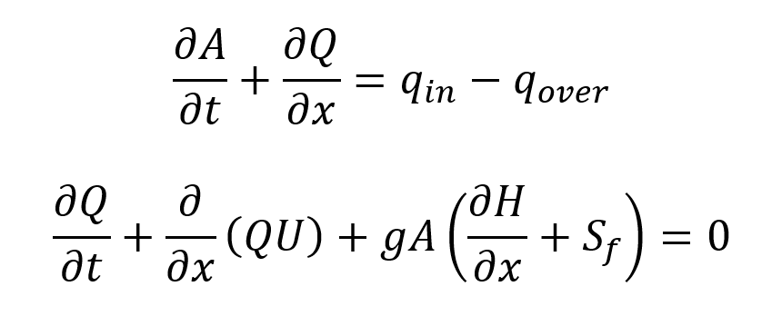
where A is the cross-sectional area of flow, Q is the flowrate, U is the average velocity of the flow, H is the hydraulic head, x is distance, t is time, qin is the lateral inflow per unit width, qover is the overflow per unit width, and Sf is the friction slope can be expressed in terms of Manning equation as:
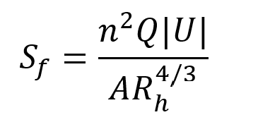
where n is the Manning roughness coefficient, and Rh is the hydraulic radius of flow cross section. Surcharged flow conditions in closed conduits are modeled using Preissmann Slot (Preissmann, 1961) and Dynamic Preissmann Slot (Sharior et al., 2023).
The discretization of the SVEs is essential for obtaining stable and accurate results under a wide variety of flow conditions. The staggered-grid scheme, which is conceptually different from four-point implicit schemes, discretizes and solves the SVEs in a series of staggered control volumes, while four-point schemes solve for flows and heads at the same locations. Furthermore, FSGI utilizes recurrence relations, significantly reducing the size of the sparse solution matrix so that considerable savings in computational effort are realized compared to more conventional four-point implicit schemes. This is accomplished without omitting any terms of the SVEs under either supercritical or subcritical flow conditions, ensuring accurate results during transitions between hydraulic states.
SWMM6 alpha introduces several updates to the SWMM5 dynamic wave framework while retaining the general SWMM5 link-node solution structure. The updates considered in this paper are the semi-implicit node continuity formulation, Anderson acceleration for Picard iteration, and the Dynamic Preissmann Slot surcharge option. These methods are intended to improve numerical robustness, nonlinear convergence, and surcharge-transition behavior relative to SWMM5 Dynamic Wave, without changing the solver into a fully coupled global implicit formulation.
Semi-Implicit Node Continuity:
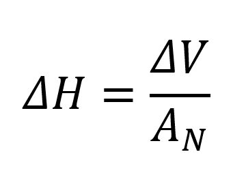
SWMM6 alpha adds an optional semi-implicit node continuity formulation to reduce the oscillations that can occur when a node transitions between free-surface and surcharged conditions. In the legacy SWMM5 dynamic wave formulation, the node-depth update uses different logic depending on whether the node is surcharged. For non-surcharged conditions, the node depth correction is based primarily on the available surface area:
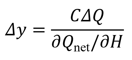
where C is a coefficient, ΔQ is the flow imbalance, and ∂Qnet /∂H is the derivative of net flow with respect to hydraulic head.
Both update formulas are reasonable within their own hydraulic regimes. The numerical weakness occurs at the transition between the two regimes. Near the conduit crown, a node can switch back and forth between the free-surface branch and the surcharged branch during successive iterations or timesteps. This branch switching can produce head oscillations that often require smaller routing timesteps or additional damping in SWMM5-style dynamic wave simulations.
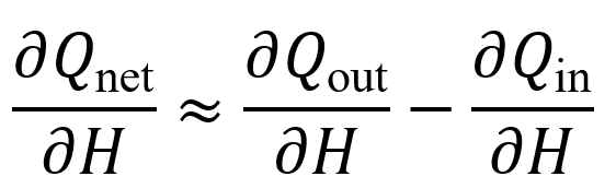
The SWMM6 semi-implicit formulation removes this discrete branch switching by using a single continuity equation for both regimes. Instead of using a purely explicit forward update, SWMM6 applies a Crank–Nicolson, or trapezoidal, time discretization. The net flow is averaged between the old and new states. The resulting unified node-depth correction is:
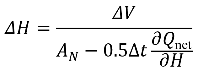
This equation blends the free-surface storage term, (AN), with the surcharged-flow sensitivity term, (∂Qnet/∂H). When the node is clearly free-surface, the surface-area term dominates, and the update behaves like the legacy free-surface correction. When the node is surcharged, the flow-head sensitivity term becomes more important. Near the transition, both terms contribute simultaneously, producing a smoother update without switching between two separate formulas.
When ∂Qnet/∂H=0, the semi-implicit update reduces to the legacy SWMM5-style node continuity update. When (SH) is large, the denominator increases and the resulting depth correction is reduced. This gives the node update additional numerical damping during surcharge transitions and other hydraulically stiff conditions.
Anderson Acceleration for Picard Iteration:
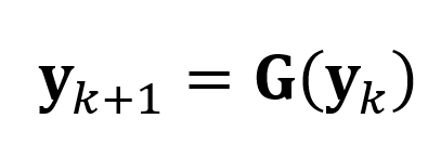
SWMM6 alpha adds Anderson acceleration as a convergence enhancement to the existing Picard iteration used in the dynamic wave solver. The dynamic wave solution can be viewed as a fixed-point problem in which the solver repeatedly updates the vector of nodal depths until the change between iterations satisfies the head tolerance:
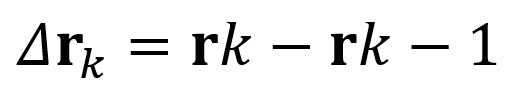
and the mixing coefficient is computed as:
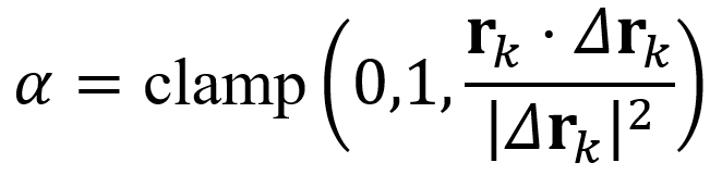
The accelerated depth estimate is then:
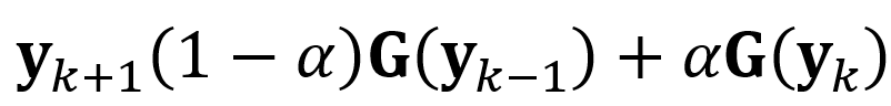
This formulation selects a weighted combination of the two most recent under-relaxed Picard outputs to reduce the remaining fixed-point residual. When α=1, the method reduces to the ordinary Picard update. When 0 < α < 1, the update uses recent residual history to move more directly toward the fixed point.
In SWMM6 alpha, Anderson acceleration is used as a local convergence accelerator rather than a reformulation of the dynamic wave equations. It does not assemble a Jacobian and does not convert the SWMM5 dynamic wave solver into a fully implicit matrix solution. The implementation also includes safety guards that revert selected nodes to the standard Picard update when the residual is too large, the accelerated depth is nonphysical, or the hydraulic update is discontinuous because of pumps, weirs, or surcharge-transition logic. Therefore, Anderson acceleration improves nonlinear convergence behavior while preserving the underlying SWMM5 link-node iteration structure.
Justification for the use of any numerical scheme rests on its efficiency and stability in solving practical problems by means of computer implementation. More specifically, SWMM5, SWMM6 alpha, and FSGI are coded in AquaTwin Sewer and can be tested using identical input data and equivalent accuracy tolerances. The efficacy of these methods is illustrated here by application to the SWMM5 QA/QC test cases and to one actual sewer collection system. Results show that FSGI consistently outperforms SWMM5 and SWMM6 alpha in terms of computational stability, accuracy, and speed.

Figure 1: Profile view of TEST 1.
The first hydraulic challenge example network is a flat run of pipe. The profile of the pipe layout is shown in Figure 1. The network comprises ten 100-ft-long, 4-ft-diameter circular pipes placed on a flat (0%) slope. The network is subjected to a 3-hour square-wave inflow hydrograph of 100 cfs magnitude at the upstream end and was run for a 5-hour simulation period using 5-second and 120-second routing timesteps.
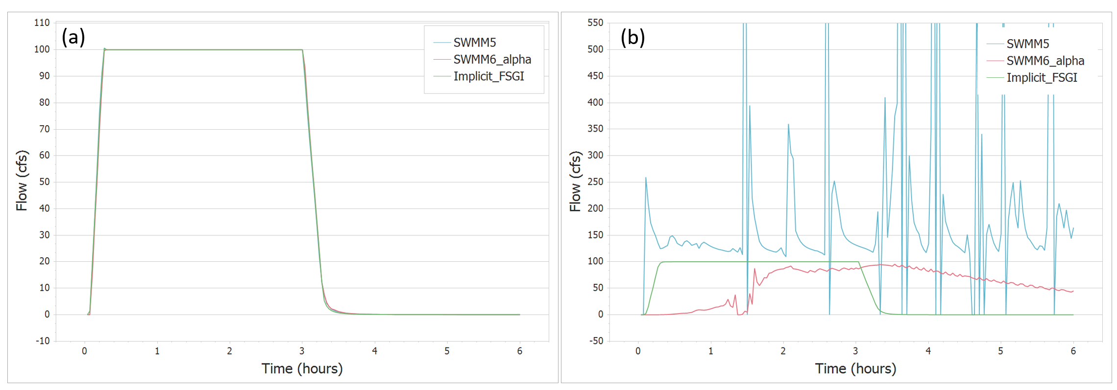
Figure 2: TEST 1 flowrate comparisons for link 9 between SWMM5, SWMM6 alpha and Implicit FSGI for a routing timestep of (a) 5 seconds and (b) 120 seconds.
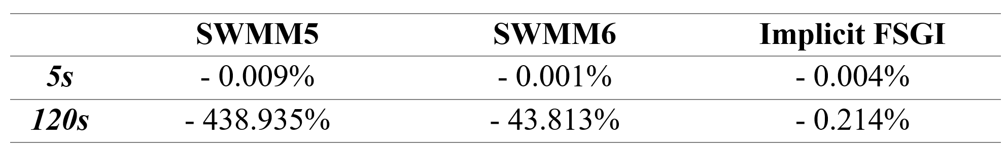
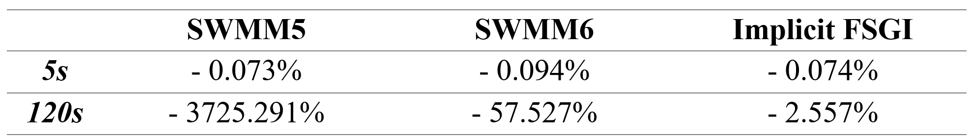
Figure 2 shows the flowrate in link 9 for SWMM5, SWMM6, and Implicit FSGI for 5-second and 120-second routing timesteps. For the 5-second routing timestep, SWMM5, SWMM6, and Implicit FSGI are stable, and the flowrates are virtually identical. For the 120-second routing timestep, both SWMM5 and SWMM6 are completely unstable, while Implicit FSGI is stable and conserves mass. The mass balance errors are reported below.
Table 1: TEST 1 mass balance error comparison
The next hydraulic challenge test network represents a pipe constriction subjected to surcharge. The profile of the pipe layout is shown in Figure 3. It consists of alternating sections of 12-ft-diameter circular pipe flowing into a 3-ft-diameter pipe. Each section is 1,000 ft long and has a slope of 0.05%. The inflow hydrograph to the system is a 50 cfs, 3-hour square-wave pattern. The system was run for a 6-hour duration using 5-second and 120-second routing timesteps.
Figure 4 depicts the flowrate in link 3 for SWMM5, SWMM6, and Implicit FSGI for 5-second and 120-second routing timesteps. For the 5-second routing timestep, both SWMM5 and SWMM6 show signs of instability while Implicit FSGI is completely stable. For the 120-second routing timestep, SWMM5 is completely unstable. Although SWMM6 appears stable based on its relatively low continuity error (-2.561%), it heavily distorts the overall shape of the routed flow hydrograph. In contrast, Implicit FSGI remains stable, conserves mass and preserves the shape of the routed hydrograph. The mass balance errors are reported in Table 2 below.

Figure 3: Profile view of TEST 2.
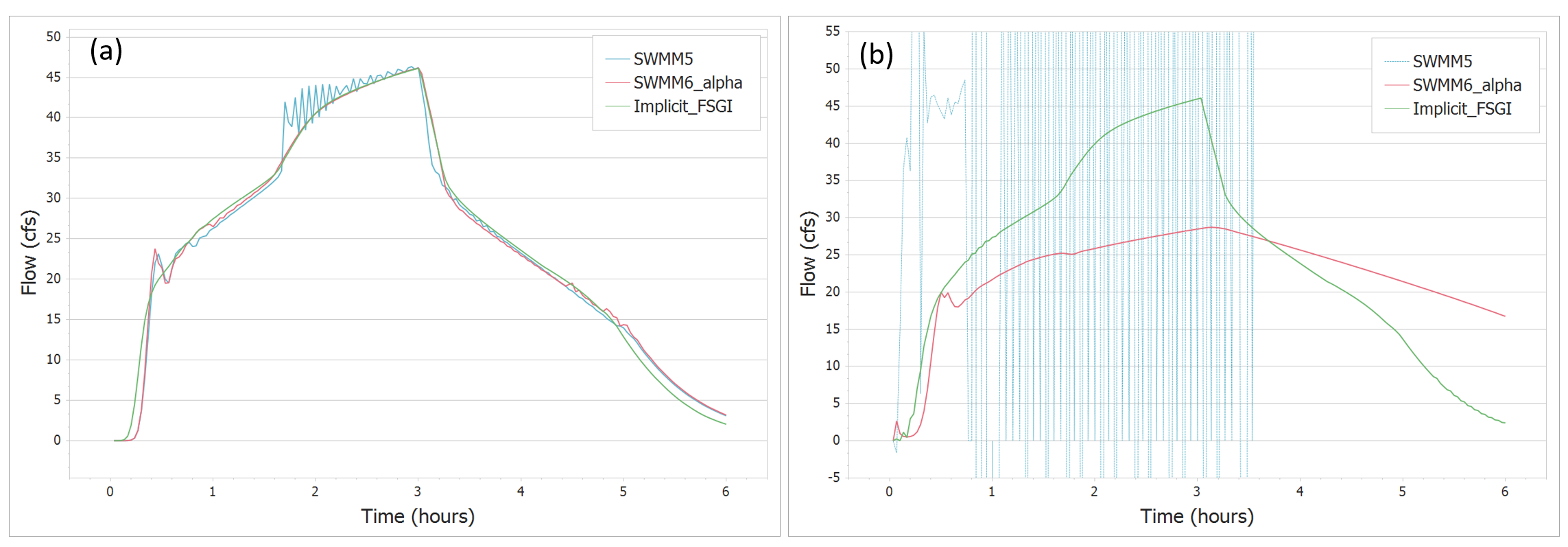
Figure 4: TEST 2 flowrate comparisons for link 3 between SWMM5, SWMM6 and Implicit FSGI for a routing timestep of (a) 5 seconds and (b) 120 seconds.
Table 2: TEST 2 mass balance error comparison


Figure 5: Profile view of TEST 3.
This example network is shown in Figure 5 and consists of six sections of 6-ft-diameter circular pipe that drop 40 ft to connect with another six sections of 3-ft-diameter pipe. Each section is 500 ft long with a slope of 0.10%. Junction 7 has an invert discontinuity resulting in a 32-ft drop. The simulation was carried out for a 6-hour duration using 5-second and 120-second routing timesteps.
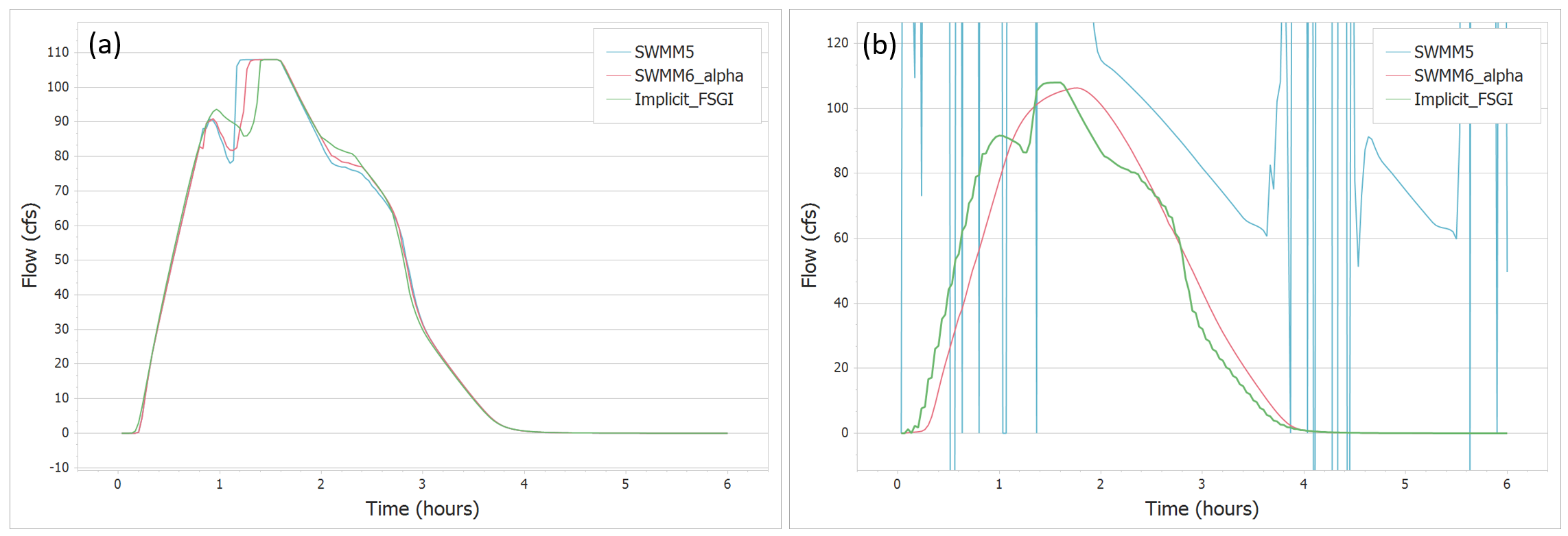
Figure 6: TEST 3 flowrate comparisons for link 105 between SWMM5, SWMM6 and Implicit FSGI for a routing timestep of (a) 5 seconds and (b) 120 seconds.
Figure 6 depicts the flowrate in link 105 for SWMM5, SWMM6, and Implicit FSGI for 5-second and 120-second routing timesteps. For the 5-second routing timestep, both SWMM5 and SWMM6 show signs of instability while Implicit FSGI is completely stable. For the 120-second routing timestep, SWMM5 is completely unstable. Similar to Test 2, SWMM6 appears stable from the continuity-error summary; however, it heavily distorts the routed hydrograph by smoothing important hydraulic details. Implicit FSGI is completely stable and conserves mass. The mass balance errors are reported below.
Table 3: TEST 3 mass balance error comparison
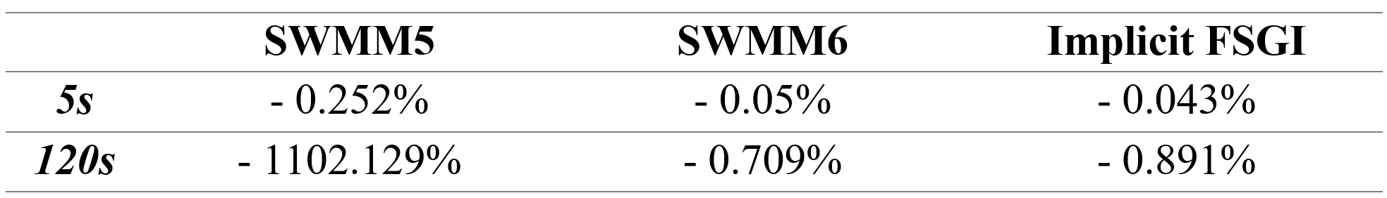
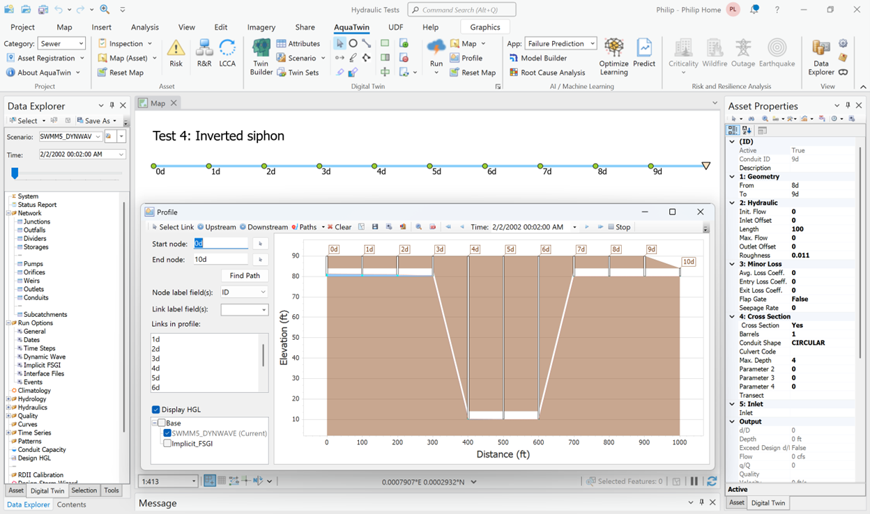
Figure 7: Profile view of TEST 4.
This example network is an inverted siphon, and the profile is shown in Figure 7. All conduits are 100-ft-long, 4-ft-diameter circular pipes. The inflow hydrograph is a 3-hour square wave of 100 cfs magnitude. The system was run for a 5-hour duration using 5-second and 120-second routing timesteps.
Figure 8 depicts the flowrate in link 5 for SWMM5, SWMM6, and Implicit FSGI for 5-second and 120-second routing timesteps. For the 5-second routing timestep, all three engines are stable. For the 120-second routing timestep, both SWMM5 and SWMM6 are unstable, whereas Implicit FSGI is stable and conserves mass. The mass balance errors are reported in the table below.
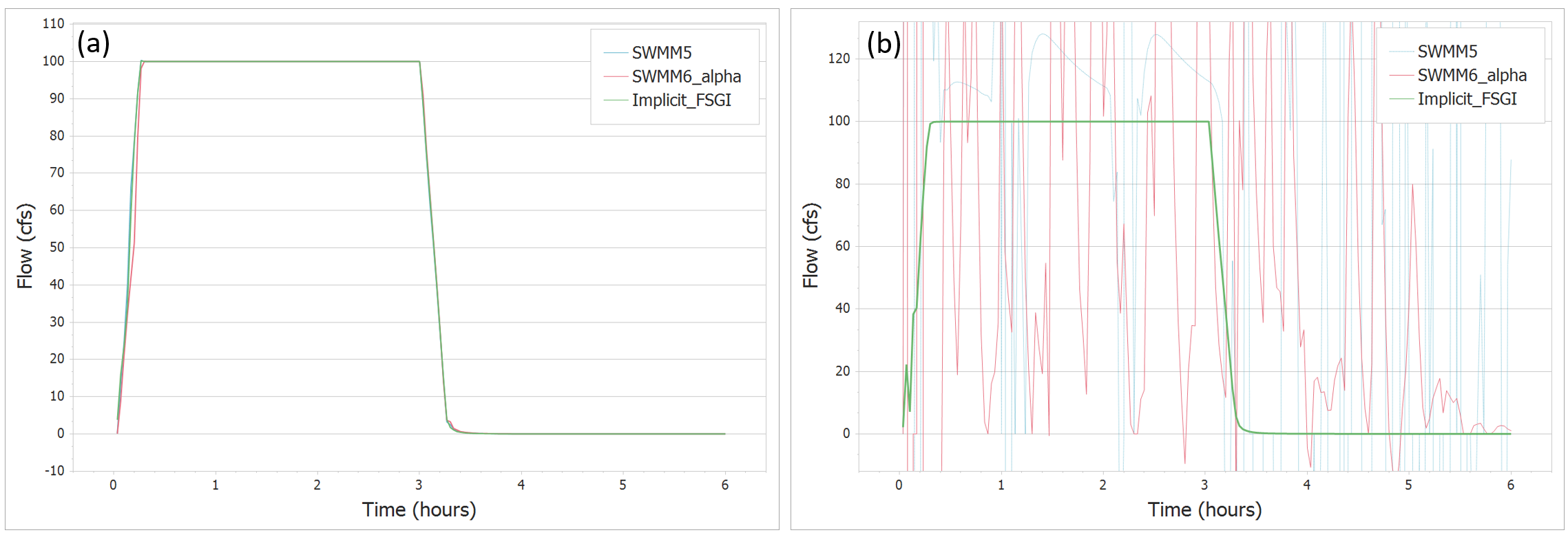
Figure 8: TEST 4 flowrate comparisons for link 5 between SWMM5, SWMM6 and Implicit FSGI for a routing timestep of (a) 5 seconds and (b) 120 seconds.
Table 4: TEST 4 mass balance error comparison
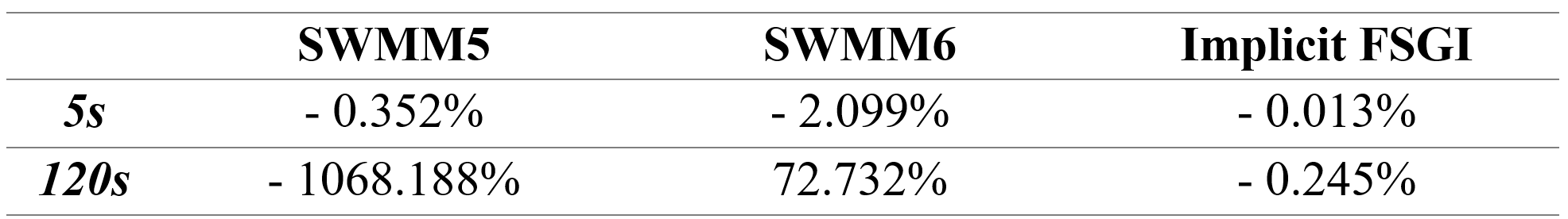
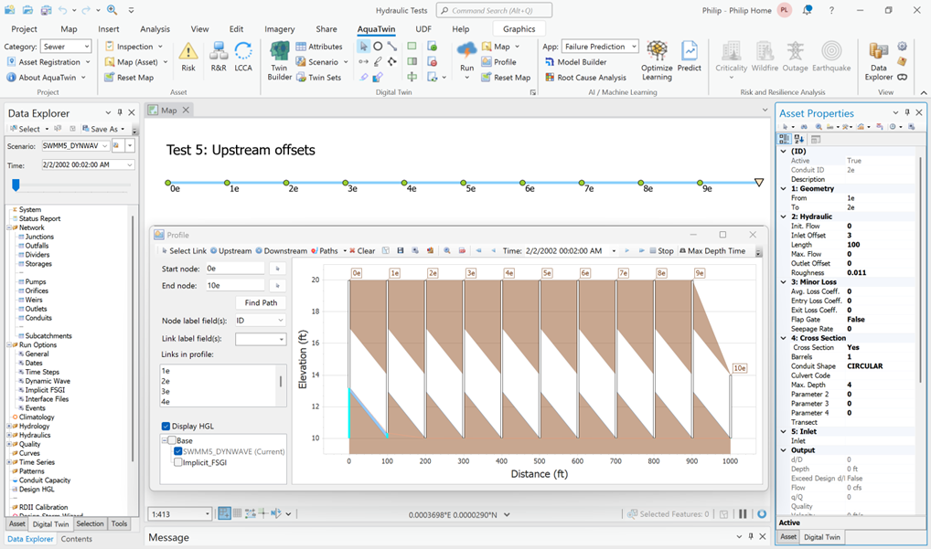
Figure 9: Profile view of TEST 5.
The final hydraulic challenge test network is a sequence of conduits, each of which has a 3-ft offset from the invert of its inlet node. Each conduit is a 100-ft-long, 4-ft-diameter circular pipe at a 3% slope. The profile of this layout is shown in Figure 9. The simulation was run for a 12-hour duration using 5-second and 120-second routing timesteps.
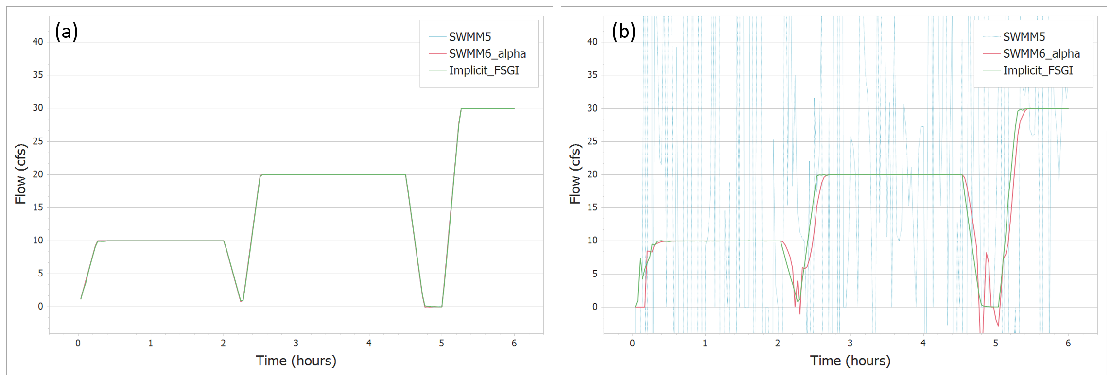
Figure 10: TEST 5 flowrate comparisons for link 1 between SWMM5, SWMM6 and Implicit FSGI for a routing timestep of (a) 5 second and (b) 120 second.
Figure 10 depicts the flowrate in link 1 for SWMM5, SWMM6, and Implicit FSGI for 5-second and 120-second routing timesteps. For the 5-second routing timestep, SWMM5, SWMM6, and Implicit FSGI are stable. However, SWMM5 and SWMM6 are unstable for the 120-second routing timestep, whereas Implicit FSGI is stable and conserves mass. The mass balance errors are reported below.
Table 5: TEST 5 mass balance error comparison
We now analyze the eight EXTRAN test cases described in the SWMM5 QA/QC report (Rossman, 2006). These network layouts are shown in Figure 11. These EXTRAN test cases were run with 20-second and 900-second routing timesteps.
For the 20-second routing timestep, SWMM5, SWMM6, and Implicit FSGI results are stable, and the mass balance error is within an acceptable range. However, SWMM5 and SWMM6 are completely unstable for the 900-second routing timestep, while Implicit FSGI is stable and conserves mass. The resulting mass balance error comparison for the 900-second routing timestep simulations for the EXTRAN networks is presented in Table 6.
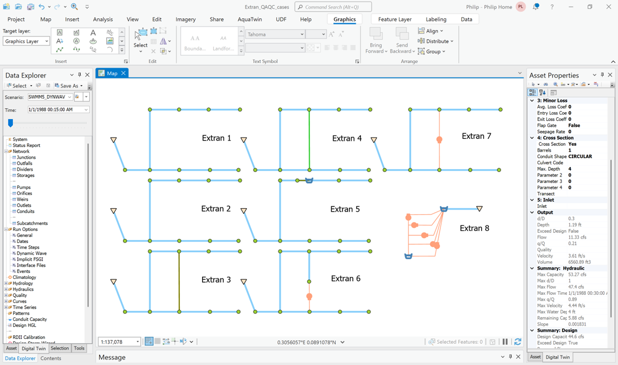
Figure 11: Network layout of the EXTRAN test cases.
Table 6: EXTRAN networks mass balance error comparison
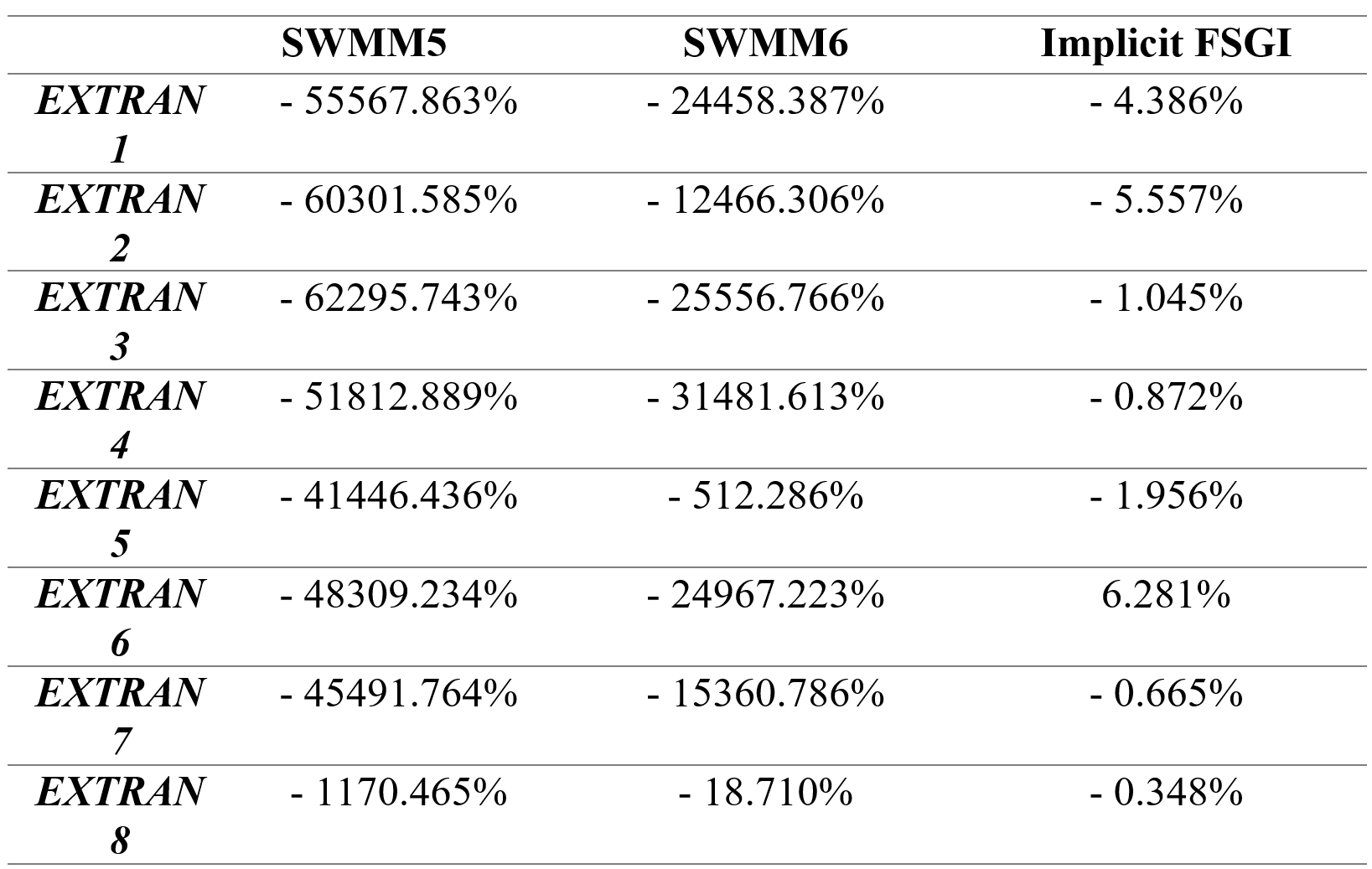
Table 6 clearly demonstrates that Implicit FSGI is completely stable and effectively conserves mass for the eight EXTRAN networks, even for a very large 900-second routing timestep.
USER 1 network is shown in Figure 12 and consists of a 175-hectare drainage area divided into 58 subcatchments. The conveyance system contains 59 circular conduits connected to 59 junctions and a single outfall. The elevation profile of the main stem drops almost 19 m over 2.5 km. The hydraulic simulation was carried out using 5-second and 60-second flow routing timesteps for a 7-hour duration with a 1-minute reporting timestep.
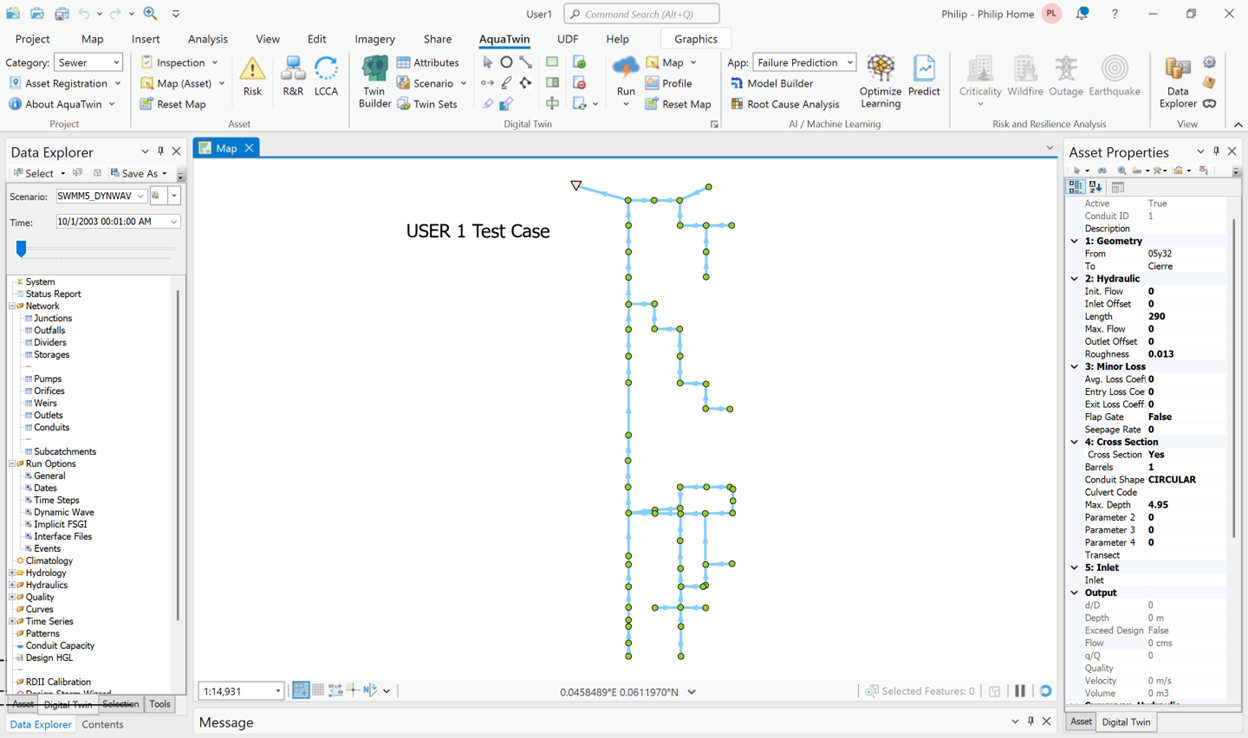
Figure 12: Network layout of the USER 1 test case.
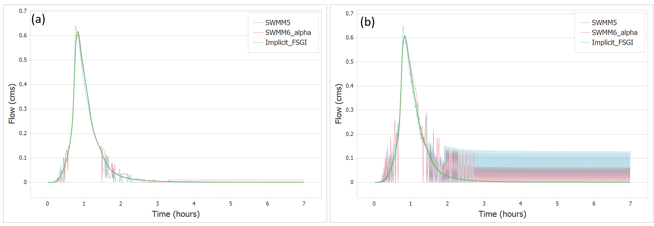
Figure 13: USER 1 flowrate comparisons for link 50 between SWMM5, SWMM6 and Implicit FSGI for a routing timestep of (a) 5 seconds and (b) 60 seconds.
Most of the links and nodes for the SWMM5 and SWMM6 solvers are stable for a 5-second routing timestep. However, signs of instability are seen in link 50. Implicit FSGI is completely stable at the 5-second routing timestep, as depicted in Figure 13(a). For the 60-second routing timestep, SWMM5 and SWMM6 are completely unstable, whereas Implicit FSGI maintains stability, as shown in Figure 13(b). The resulting mass balance error comparison is given in Table 7 below.
Table 7: USER 1 mass balance error comparison
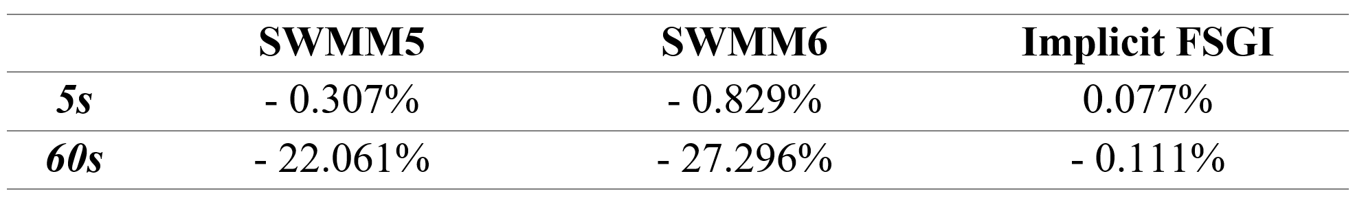
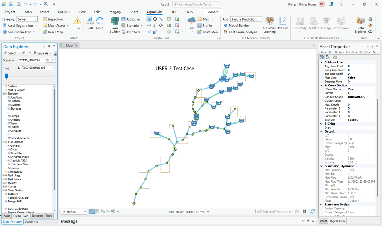
Figure 14: Network layout of the USER 2 test case.
This example network is shown in Figure 14 and consists of a 3.5-square-mile drainage area broken into 17 subcatchments. The network comprises 83 conduits that are a mixture of irregular natural channels, open channels, and closed pipes of various shapes. There are 28 storage units along with 19 weirs. Many of these storage units and weirs represent junctions with above-ground surface storage coupled with road overflows. A 4.4-inch, 24-hour design storm is applied to the network over a 36-hour simulation period using 5-second and 30-second flow routing timesteps with a 5-minute reporting timestep.
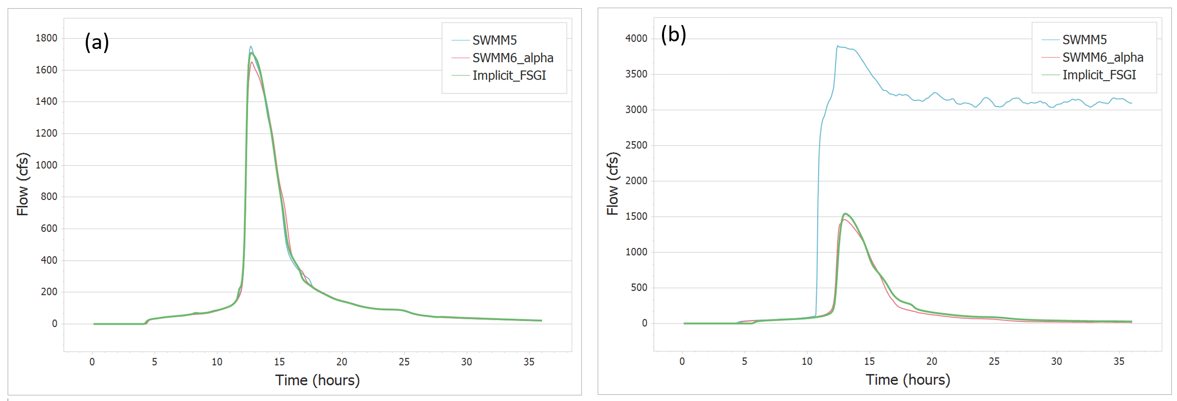
Figure 15: USER 2 flowrate comparisons for outfall link TW01020 between SWMM5, SWMM6 and Implicit FSGI for a routing timestep of (a) 5 seconds and (b) 30 seconds.
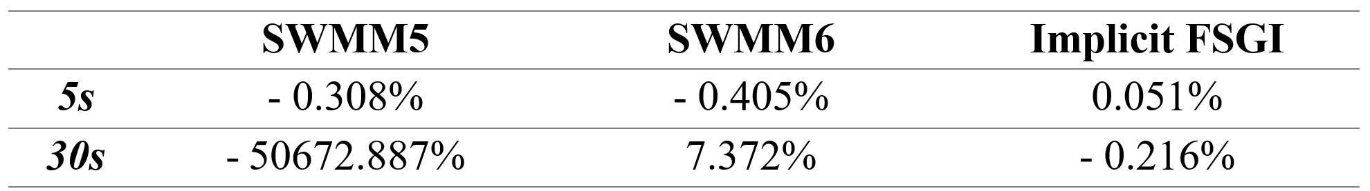
SWMM6 slightly underpredicts the flowrate at the outfall link TW01020, resulting in the highest continuity error at a 5-second routing timestep, as depicted in Figure 15(a), while SWMM5 and Implicit FSGI conserve mass better. At the 30-second routing timestep, SWMM5 is completely unstable. SWMM6 performs better than SWMM5, resulting in a lower continuity error, but it shows the general characteristic of changing the shape of the hydrograph. Implicit FSGI is completely stable at the 30-second routing timestep, and the mass balance error is only -0.216%.
Table 8: USER 2 mass balance error comparison
The USER 3 network is a combined sewer system comprising 168 subcatchments that encompass an area of 6 km². The network schematic is shown in Figure 16. The system contains 134 pipes of mostly circular or egg-shaped cross sections. Of the 141 nodes in the network, 6 are outfalls and 130 are manhole or catch basin structures represented as small storage units. There are 5 pumps in the network that discharge directly to the system outfalls. A 3-hour, 42 mm design storm is used in the simulation. This network was originally assessed using a 0.5-second routing timestep with a 1-minute reporting timestep for a 6-hour total duration.
At a very small 0.5-second routing timestep, both SWMM5 and SWMM6 are stable, resulting in mass balance errors of -0.023% and -0.092%, respectively. However, both SWMM5 and SWMM6 show signs of instability even with relatively low continuity errors, as shown in Figure 17(a). For the same routing timestep, Implicit FSGI is also stable with -0.063% mass balance error. The Implicit FSGI solver is also stable at a large 120-second routing timestep, resulting in a mass balance error of 2.499%. However, SWMM5 is completely unstable at the 120-second routing timestep, resulting in a mass balance error of -620.360%. Compared to SWMM5, SWMM6 is relatively stable with a continuity error of -8.599%; however, it shows the general characteristic of changing the shape of the hydrograph. The effects of large routing timesteps on the stability of SWMM5, SWMM6, and Implicit FSGI are shown in Figure 17.
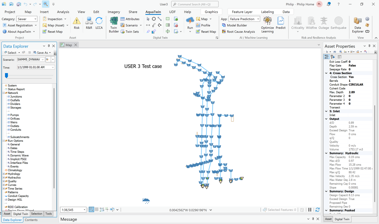
Figure 16: Network layout of the USER 3 test case.
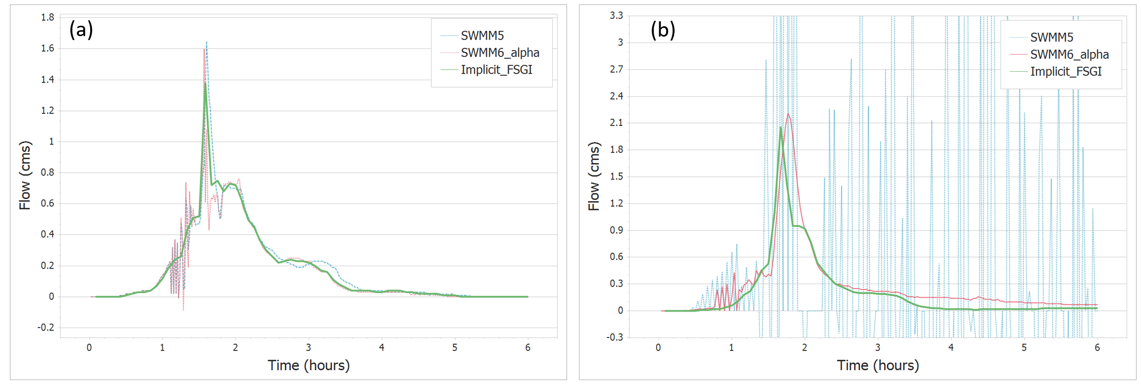
Figure 17: USER 3 flowrate comparisons for link CELCING between SWMM5, SWMM6 and Implicit FSGI for a routing timestep of (a) 0.5 seconds and (b) 120 seconds.
USER 4 network is a combined sewer system covering 528 acres divided into 112 subcatchments. The network schematic is shown in Figure 18. There are 209 circular conduits connecting 209 junctions and one outfall. Each subcatchment contributes both a dry-weather sanitary flow, modeled as an external time series inflow applied to the subcatchment outlet node, and a wet-weather flow produced by the storm. The system is analyzed over a 24-hour simulation period using 1-second, 10-second, and 15-second flow routing timesteps with a 5-minute reporting timestep.
With a 1-second routing timestep, both SWMM5 and SWMM6 are stable with mass balance errors of -2.301% and -3.230%, respectively. For the same 1-second routing timestep, Implicit FSGI is also stable with a much better mass balance error of -0.05%. At a 10-second routing timestep, both SWMM5 and SWMM6 are completely unstable with excessively high mass balance errors of -2979.022% and -38.496%, respectively. In contrast, Implicit FSGI is stable at a 15-second routing timestep with an excellent mass balance error of 0.108%. The effect of a larger routing timestep on the stability of SWMM5 and SWMM6 is shown in Figure 19.
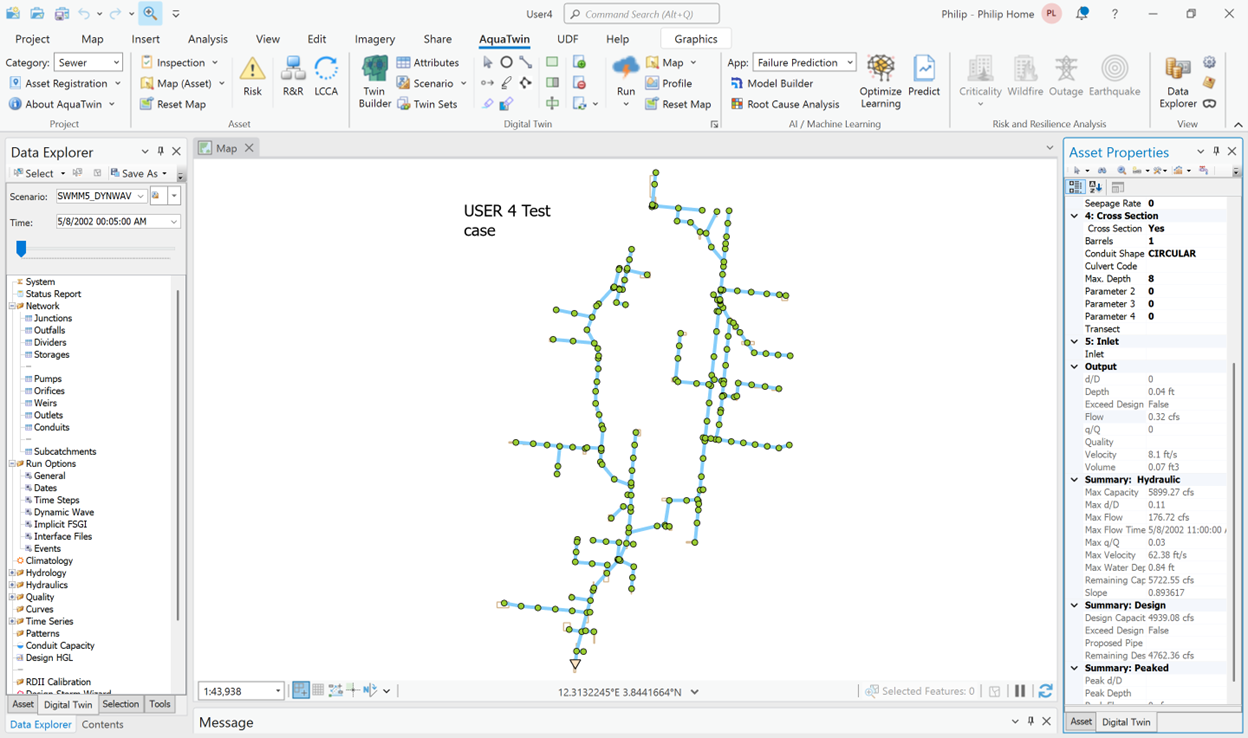
Figure 18: Network layout of the USER 4 test case.
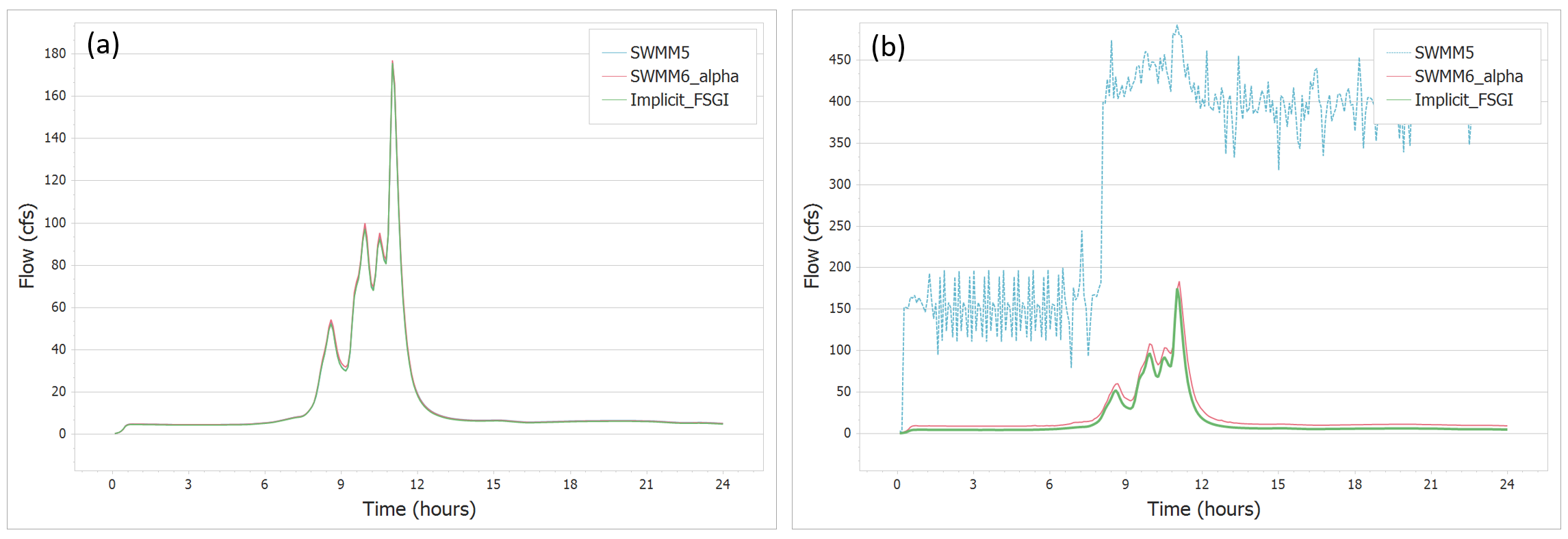
Figure 19: USER 4 flowrate comparisons for link 3701005-23701001 between SWMM5, SWMM6 and Implicit FSGI for a routing timestep of (a) 0.5 second and (b) 120 seconds.
The USER 5 network represents a 1,177-acre watershed using 145 subcatchments draining to 273 conduits, the majority of which are irregular natural channels. The drainage system schematic is shown in Figure 20. A design storm event is routed through this network. In addition, the network receives inflows at 3 locations from upper portions of the watershed that are modeled separately. The network is analyzed over a 4-hour period using a 1-minute reporting timestep and 0.5-second and 5-second flow routing timesteps.
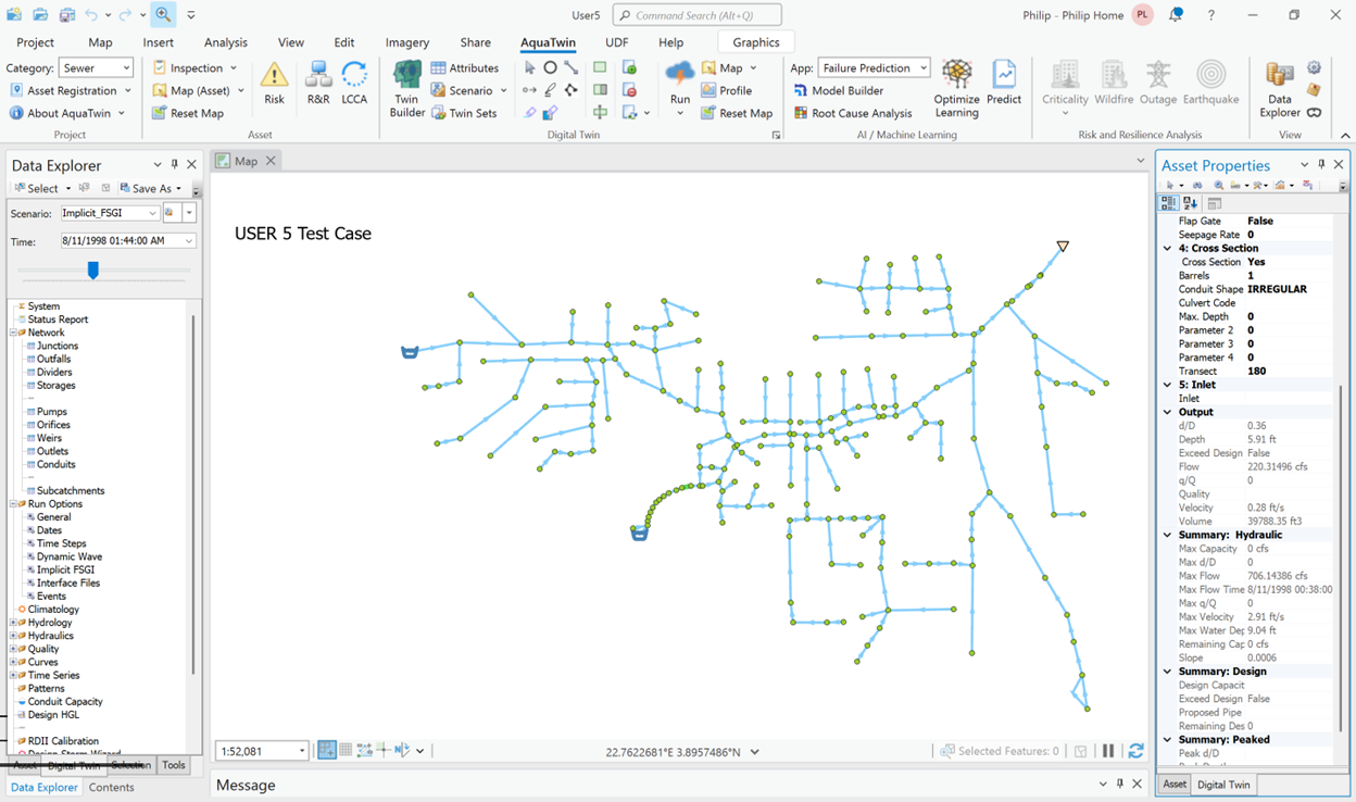
Figure 20: Network layout of the USER 5 test case.
At a 0.5-second routing timestep, both SWMM5 and SWMM6 result in reasonable mass balance errors of -0.907% and 1.183%, respectively. However, model instability and large flow oscillations are seen throughout the network despite the relatively small balance errors, as depicted in Figure 21(a) and (b). Implicit FSGI with the same 0.5-second routing timestep resulted in a stable simulation with a mass balance error of -0.717%. At a 5-second routing timestep, both SWMM5 and SWMM6 exhibit more instability with significant flow oscillations. However, Implicit FSGI produces stable and smooth solutions.
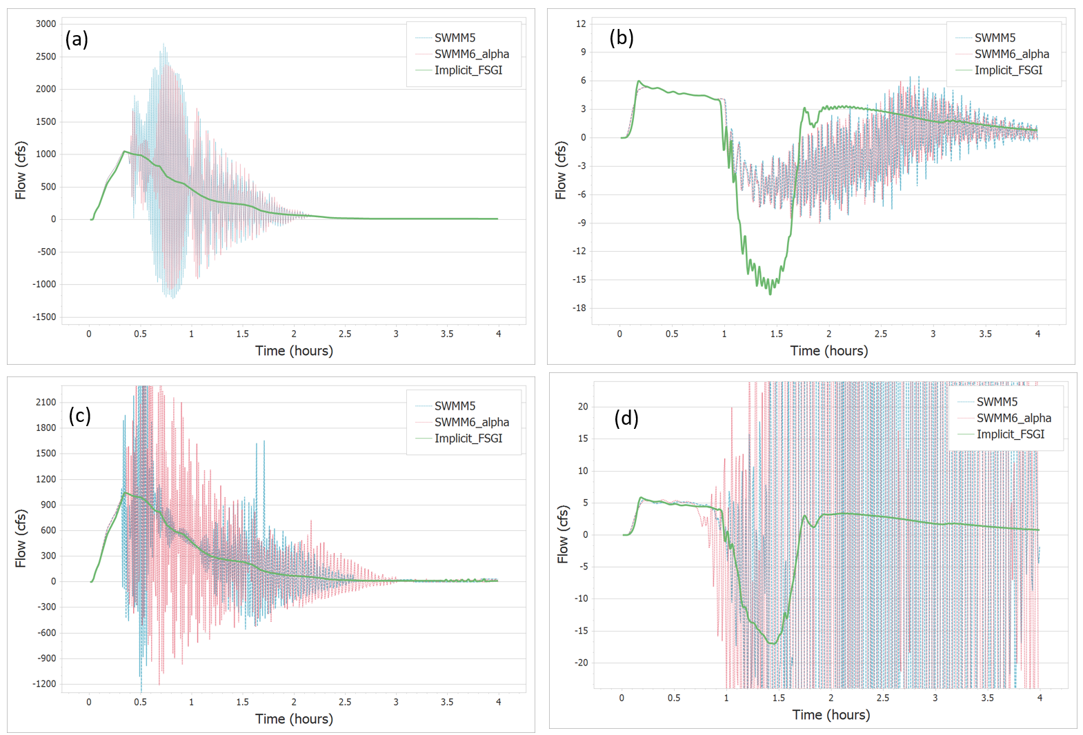
Figure 21: USER 5 flowrate comparisons for (a) link LIB_1 for a routing timestep of 0.5 second, (b) link 626 for a routing timestep of 0.5 second, (c) link LIB_1 for a routing timestep of 5 seconds, and (d) link 626 for a routing timestep of 5 seconds between SWMM5, SWMM6 and Implicit FSGI for a routing timestep of (a) 0.5 second and (b) 5 seconds.
The actual Sewer Network_1 is a large and complex actual sewer network. It consists of 5,818 conduits, 5,637 junctions, 115 storage units, 31 pumps, 42 orifices, and 101 weirs spread over 4,375 subcatchments. In addition, this network has sophisticated pumps, weirs, and orifice controls. CDM Smith provided this network for testing, and this test case has been used here to benchmark simulation runtimes between SWMM5, SWMM6, and Implicit FSGI. The network is analyzed over a 24-hour simulation period using a 15-minute reporting timestep.
Using a 15-second variable routing timestep, the SWMM5 simulation completed in 4 minute and 15 seconds with a mass balance error of -0.526%. Under the same timestep setting, SWMM6 completed the simulation in 2 minute and 48 seconds with a mass balance error of -0.610%. This represents an approximate 34% reduction in runtime for SWMM6 relative to SWMM5, primarily due to the improved nonlinear convergence provided by Anderson acceleration.

Figure 22: Network layout of the Real Sewer Network_1 test case.
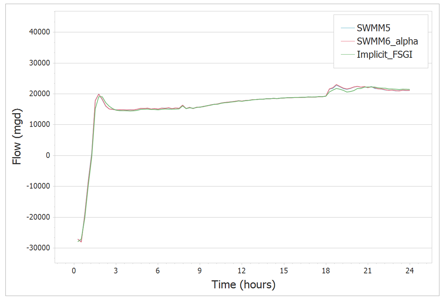
Figure 23: Flowrate comparisons for the outfall link for Actual Sewer Network_1 between SWMM5, SWMM6 and Implicit FSGI.
Implicit FSGI produced virtually identical hydraulic results while using a larger 30-second fixed routing timestep. The Implicit FSGI simulation completed in 29 seconds with an improved mass balance error of 0.279 %. Thus, for this test case, Implicit FSGI was approximately 9 times faster than SWMM5 and 6 times faster than SWMM6, while maintaining comparable hydraulic behavior with better mass conservation.
This white paper compares SWMM5, SWMM6 alpha, and Implicit FSGI for one-dimensional dynamic sewer and channel network modeling using the SWMM5 QA/QC benchmark suite and one large actual sewer network. The QA/QC cases included hydraulic challenge tests, EXTRAN control networks, and user test networks representing surcharge, conduit constrictions, drop structures, inverted siphons, offset conduits, hydraulic controls, and complex drainage-system behavior. The results show that SWMM6 alpha is generally an improvement over SWMM5. In many of the QA/QC cases, SWMM6 alpha reduced the severity of continuity errors relative to SWMM5, particularly at larger routing timesteps. This improvement is consistent with the numerical updates introduced in SWMM6 alpha, including the semi-implicit node continuity formulation, Anderson acceleration for Picard iteration, and the Dynamic Preissmann Slot surcharge option.
However, the SWMM6 alpha results should be interpreted with caution. A small continuity error by itself does not guarantee that the routed hydrograph is hydraulically accurate. Several test cases show that SWMM6 alpha can produce lower mass-balance error than SWMM5 while still distorting the shape, timing, and attenuation of the routed hydrograph. This behavior is especially evident in hydraulically challenging cases involving surcharge transitions, constrictions, drops, and large routing timesteps. In these cases, SWMM6 alpha may appear stable from the continuity-error alone, but the resulting hydrograph can be excessively smoothed, shifted in time, or otherwise altered relative to the expected hydraulic response. Therefore, SWMM6 alpha should not be evaluated using continuity error alone; hydrograph shape, peak timing, peak magnitude, and physical consistency must also be reviewed.
The large actual sewer network further reveals the practical significance of these differences. SWMM6 alpha reduced computational runtime relative to SWMM5 under the same 15-second variable routing timestep, indicating that Anderson acceleration can improve nonlinear convergence and computational efficiency. However, Implicit FSGI produced comparable hydraulic results with better mass conservation using a larger 30-second fixed routing timestep and completed the simulation significantly faster than both SWMM5 and SWMM6 alpha. This confirms the unequivocal numerical advantages of a fully implicit coupled solver for sewer and stormwater network modeling.
Implicit FSGI presents a major advancement in one-dimensional dynamic modeling of sewer and channel networks under both free-surface and surcharged conditions. By embedding the flow equations within a system of implicit linear equations, Implicit FSGI significantly improves stability, hydraulic fidelity, and computational speed. The method’s use of recurrence relations substantially reduces the size of the solution matrix, leading to faster runtimes compared to traditional implicit schemes. Extensive validation and benchmarking against SWMM5 and SWMM6 alpha, using the SWMM5 QA/QC benchmark suite and one large actual sewer network, show that Implicit FSGI provides the strongest overall performance in terms of numerical stability, timestep flexibility, hydrograph preservation, and runtime efficiency. These results demonstrate that FSGI offers a robust, reliable, mass-conservative, and efficient approach for modeling large and intricate sewer systems, making it a valuable tool for hydraulic engineers and practitioners.
Overall, SWMM6 alpha represents a minor but useful evolution of the SWMM5 Dynamic Wave framework. Its numerical updates improve some aspects of the SWMM5 legacy solver, particularly nonlinear convergence and surcharge-transition behavior, and in several cases the updates reduce continuity errors relative to SWMM5. However, SWMM6 alpha does not fundamentally change the underlying weak SWMM5 link-node solution structure, and its results must still be reviewed carefully beyond continuity error alone, especially when larger timesteps or surcharge-dominated conditions are used. Among the three methods evaluated in this study, Implicit FSGI remains the state-of-the-art and best-performing numerical approach for modeling complex sewer and stormwater networks.
Anderson, D. G. (1965). Iterative procedures for nonlinear integral equations. Journal of the ACM, 12(4), 547–560. https://doi.org/10.1145/321296.321305
Aquanuity, Inc. (2025). Comparison of fast-staggered-grid implicit and SWMM5 dynamic wave sewer network models. https://aquanuity.com/resources/comparison-of-fast-staggered-grid-implicit-and-swmm5-dynamic-wave-sewer-network-models/
Buahin, C. (2026a). Anderson acceleration for Picard iteration. LinkedIn. https://www.linkedin.com/pulse/anderson-acceleration-picard-iteration-caleb-buahin-zdlce/
Buahin, C. (2026b). New optional semi-implicit node continuity formulation for SWMM. LinkedIn. https://www.linkedin.com/pulse/new-optional-semi-implicit-node-continuity-swmm-caleb-buahin-xu0je/
Buahin, C. (2026c). A dynamic Preissmann slot for Open-Source SWMM2D. LinkedIn. https://www.linkedin.com/pulse/dynamic-preissmann-slot-open-source-swmm2d-caleb-buahin-rc8we/
Courant, R., Friedrichs, K., & Lewy, H. (1928). Über die partiellen Differenzengleichungen der mathematischen Physik. Mathematische Annalen, 100, 32–74. https://doi.org/10.1007/BF01448839
Lyn, D. A., & Goodwin, P. (1987). Stability of a general Preissmann scheme. Journal of Hydraulic Engineering, 113(1), 16–28. https://doi.org/10.1061/(ASCE)0733-9429(1987)113:1(16)
Preissmann, A. (1961). Propagation des intumescences dans les canaux et les rivières. In Proceedings of the First Congress of the French Association for Computation (pp. 433–442).
Rossman, L. A. (2006). Storm Water Management Model quality assurance report: Dynamic wave flow routing. U.S. Environmental Protection Agency.
Rossman, L. A. (2017). Storm Water Management Model reference manual, Volume II: Hydraulics (EPA/600/R-17/111). U.S. Environmental Protection Agency.
Sharior, S., Hodges, B. R., & Vasconcelos, J. G. (2023). Generalized, dynamic, and transient-storage form of the Preissmann slot. Journal of Hydraulic Engineering, 149(11), 04023045. https://doi.org/10.1061/JHEND8.HYENG-13609
Walker, H. F., & Ni, P. (2011). Anderson acceleration for fixed-point iterations. SIAM Journal on Numerical Analysis, 49(4), 1715–1735. https://doi.org/10.1137/10078356X