This white paper compares the computational performance of two different numerical methods for solving the complete one-dimensional (1D) Saint-Venant unsteady flow equations (SVEs) in sewer/channel networks. These equations consist of the continuity and momentum equations for conduits and a volume continuity equation at nodes. One method, SWMM5 Dynamic Wave (DW), is explicit in nature, while the other method, Fast Staggered-Grid Implicit (FSGI), is fully implicit. The explicit approach solves link flows and nodal heads individually using Picard’s iteration (successive approximations) scheme. The implicit approach solves link flows and nodal heads simultaneously at each time step by embedding the solutions to the SVEs into a system of implicit linear equations. The two methods are benchmarked against the well-documented 19 EPA SWMM5 QA/QC test cases under equal accuracy tolerance as well as an actual sewer system. Results show that FSGI is more computationally efficient than SWMM5 DW for sewer network modeling and generally outperforms DW by at least a factor of 8. The results also provide an insight into the limitations of SWMM5 DW in terms of numerical stability and mass conservation, problems that can be effectively overcome by FSGI.
Computational models provide the most effective and viable means of analyzing, planning, designing, operating and managing sewer collection systems. For a computational model to be useful in engineering practice, it must be very robust, accurate and efficient.
The basis of dynamic sewer modeling is the numerical solution of the 1D Saint-Venant unsteady flow equations (SVEs). There are two primary numerical methods for solving SVEs: explicit and implicit schemes. Explicit schemes are simpler and easier to formulate for sewer and channel networks. However, their inherent limitations are well known and widely documented, specifically the need for small time steps dictated by the Courant Criterion (Courant et al., 1928) resulting in excessive computational run times. Moreover, explicit schemes generally restrict conduit lengths, requiring model adjustments that can create discrepancies between the actual sewer system and the network model. Implicit schemes overcome these problems.
Though more complex, implicit schemes are unconditionally stable and improve computational speed by allowing larger time steps based on dynamic inputs rather than being limited by the Courant Criterion (Lyn & Goodwin, 1987). They also eliminate conduit length restrictions, enabling a more accurate representation of sewer networks. Generally, the four-point implicit finite difference scheme is the most widely used method for modeling sewer networks. It consists essentially of simultaneously solving linearized SVEs by means of a sparse matrix (solution matrix) routine. However, implicit schemes can become unstable under dry flow and flow reversal conditions, even under small time steps. To maintain stability, artificial base flow is often required, which in turn can cause mass balance and continuity errors.
The new Fast Staggered-Grid Implicit (FSGI) finite difference scheme improves upon traditional implicit solution schemes in terms of computational efficacy and efficiency. It solves for link flows and nodal heads simultaneously for all network elements and utilizes recurrence relations significantly reducing the size of the sparse implicit solution matrix and increasing simulation speed. Moreover, FSGI is fully mass conservative and can accurately model various geometries and flow conditions such as conduit drops, dry conduits, and backwater flows. The new FSGI scheme is validated and benchmarked against SWMM5 Dynamic Wave explicit solver (Rossman, 2017) for accuracy and efficiency using the 19 SWMM QA/QC (Rossman, 2006) test cases and an actual sewer network.
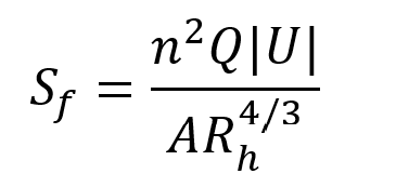
The Saint-Venant equations characterize one-dimensional, unsteady, and non-uniform flow under free-surface conditions. These equations consist of a pair of nonlinear partial differential equations dependent on both space and time. The continuity equation describes the mass balance of flow, while the momentum equation governs the balance of forces acting on the flow. They can be expressed as follows:
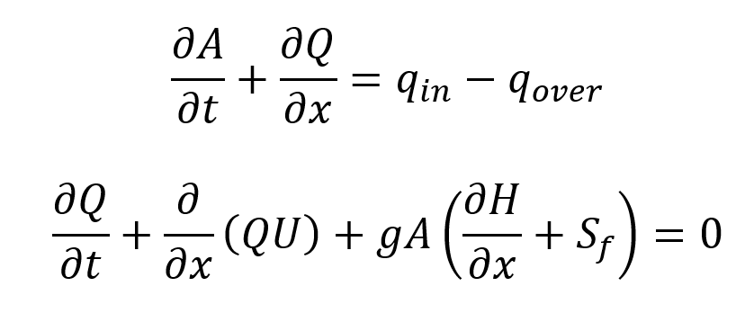
where A is the cross-sectional area of flow, Q is the flowrate, U is the average velocity of the flow, H is the hydraulic head, x is distance, t is time, qin is the lateral inflow per unit width, qover is the overflow per unit width, and Sf is the friction slope can be expressed in terms of Manning equation as:
Justification for the use of any numerical scheme rests on its efficiency and stability to solve problems by means of computer implementation. Overall, this is a comprehensive task, involving extensive analysis and investigation. More specifically, both the SWMM5 Dynamic Wave and the implicit FSGI are coded in AquaTwin Sewer and can be tested under identical input data and equal accuracy tolerances.
The computational efficacy and efficiency of the two methods are illustrated here by application to the SWMM5 QA/QC test cases and to one actual sewer collection system. Results show that FSGI consistently outperforms SWMM5 Dynamic Wave in terms of computational stability, accuracy and speed.
The first test network is a flat run of pipes. The profile of the pipe layout is shown in Figure 1. The network is comprised of ten 100-ft sections of 4-ft diameter circular pipe placed on a flat (0%) slope. The network is subjected to a 3-hour square wave inflow hydrograph of 100 cfs magnitude at the upstream node. The simulation was carried out for a 5-hour time period using 5 second and 120 second routing time steps.

Figure 1: Profile view of TEST 1.
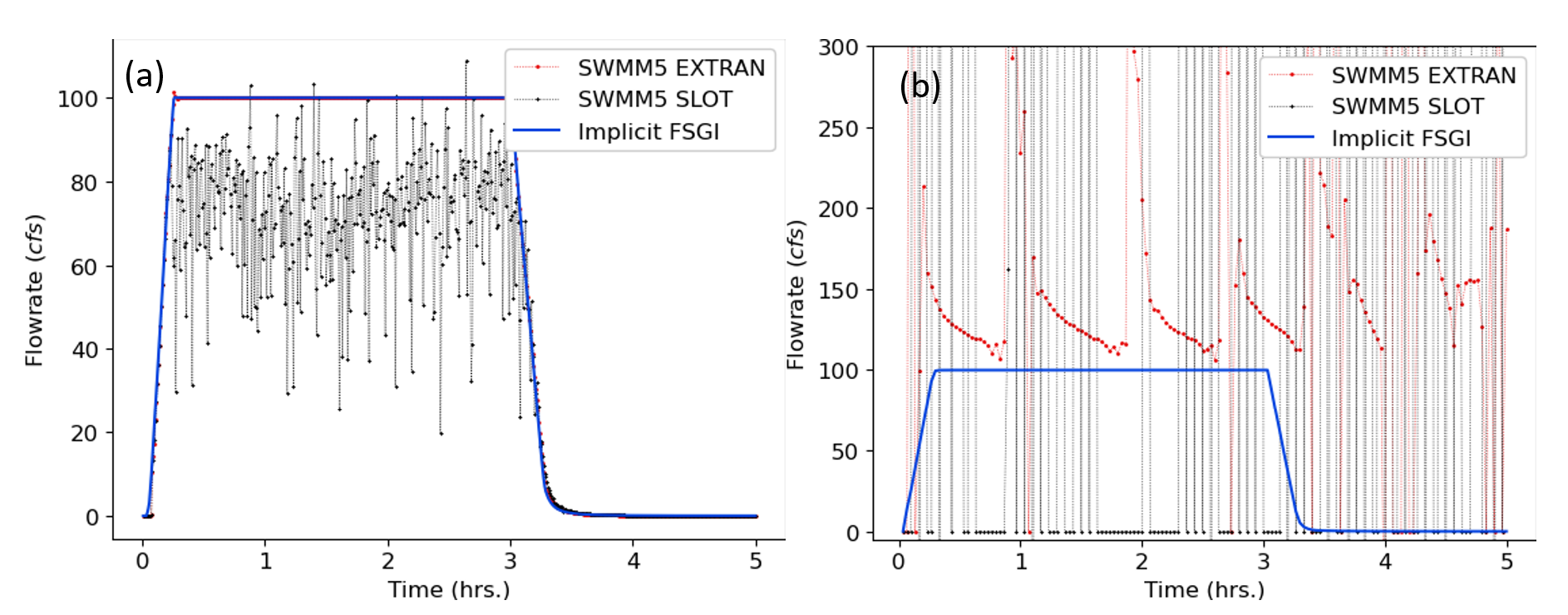
Figure 2: TEST 1 flowrate comparisons for link 9 between SWMM5 EXTRAN, SWMM5 SLOT and Implicit FSGI for a routing timestep of (a) 5 seconds and (b) 120 seconds.
Figure 2 shows the flowrate in link 9 for SWMM5 EXTRAN, SWMM5 SLOT and implicit FSGI for 5 second and 120 second routing time steps. For the 5 second routing time step, both SWMM5 EXTRAN and implicit FSGI are stable, and the flowrates are virtually identical. However, SWMM5 SLOT is unstable at a 5 second routing time step. For a 120 second routing time step, implicit FSGI was able to achieve stable results, while both SWMM5 EXTRAN and SLOT were not. Table 1 shows a detailed breakdown of mass balance errors for both scenarios.
Table 1: TEST 1 mass balance error comparison
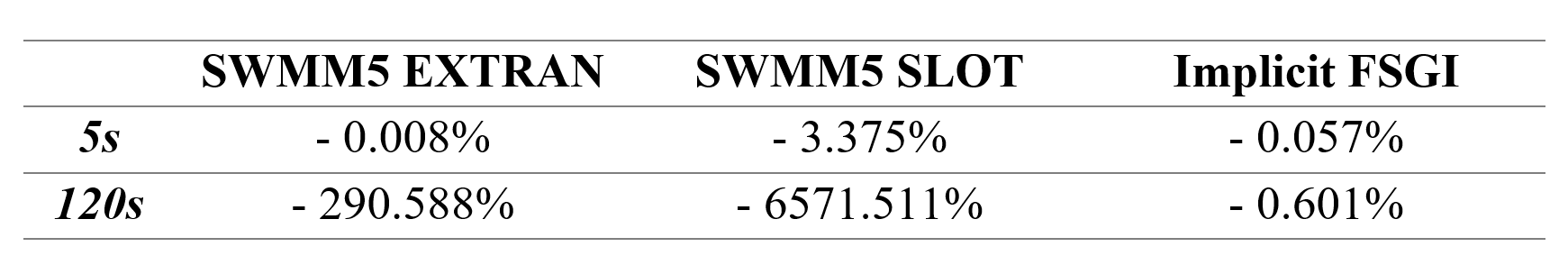

Figure 3: Profile view of TEST 2.
The next test network represents a pipe constriction that is subjected to surcharge. The profile of the pipe layout is shown in Figure 3. It consists of alternating sections of 12-ft diameter circular pipe flowing into a 3-ft diameter pipe. Each section is 1,000 ft long and has a slope of 0.05%. The inflow hydrograph to the system is a 3-hour square wave pattern with a magnitude of 50 cfs. The simulation was carried out for a 6-hour duration using 5 second and 120 second routing time steps.
Figure 4 depicts the flowrate in link 3 for SWMM5 EXTRAN, SWMM5 SLOT and implicit FSGI for 5 second and 120 second routing time steps. For the 5 second routing time step, both SWMM5 EXTRAN and SLOT shows signs of instability while implicit FSGI is completely stable. For the 120 second routing time step, both SWMM5 EXTRAN and SLOT are unstable, whereas implicit FSGI is stable and conserves mass. The mass balance errors for both scenarios are shown in Table 2.
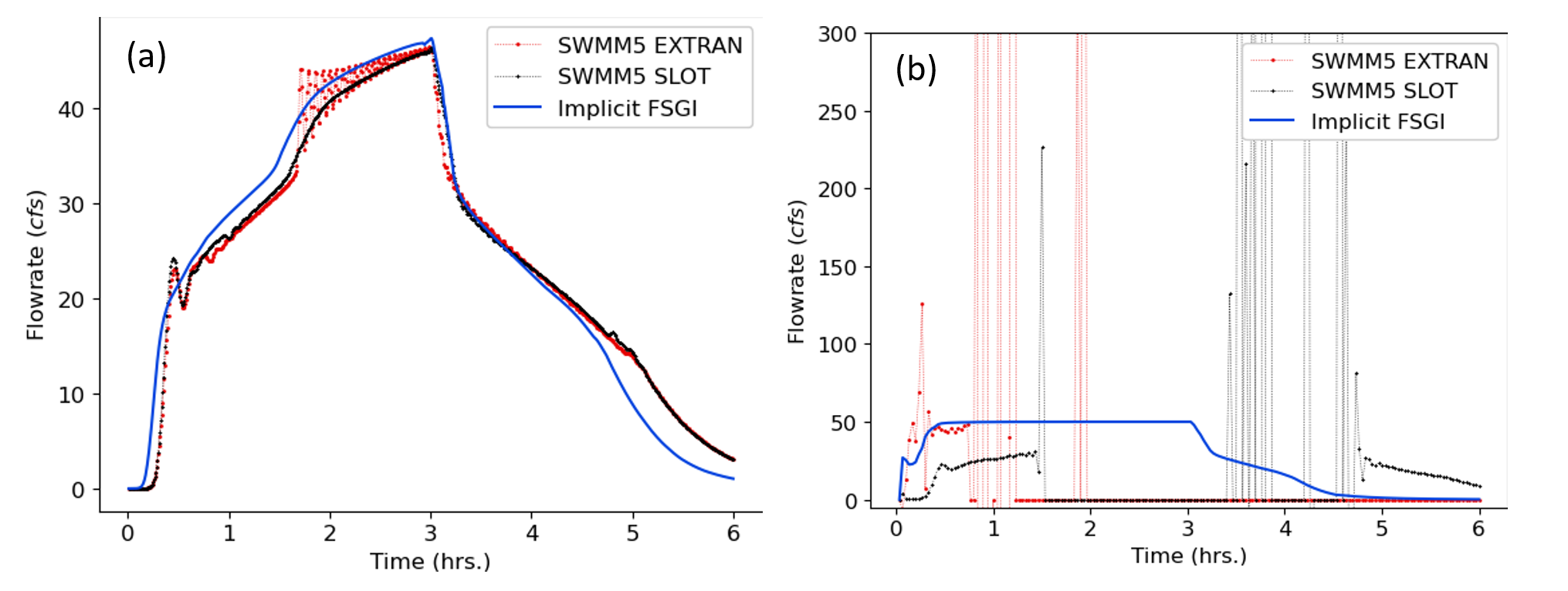
Figure 4: TEST 2 flowrate comparisons for link 3 between SWMM5 EXTRAN, SWMM5 SLOT and implicit FSGI for a routing timestep of (a) 5 seconds and (b) 120 seconds.
Table 2: TEST 2 mass balance error comparison
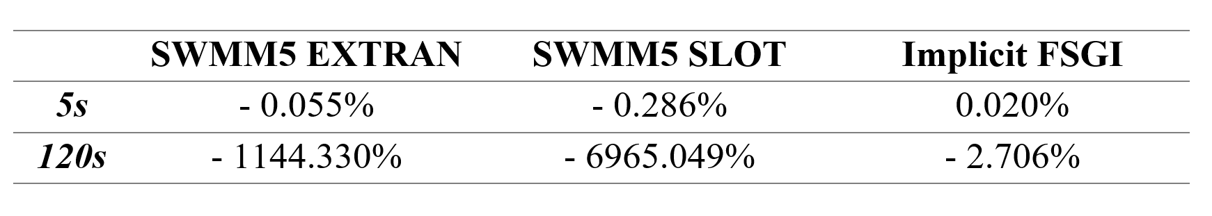

Figure 5: Profile view of TEST 3.
The next example network is shown in Figure 5 and consists of six sections of 6-ft diameter circular pipes with a 32 ft drop to connect with six sections of 3-ft diameter pipes. Each pipe section is 500 ft long with a slope of 0.10%. There is an invert discontinuity at Junction 7 resulting in a 32 ft drop. The simulation was carried out for a 6-hour duration using 5 second and 120 second routing time steps.
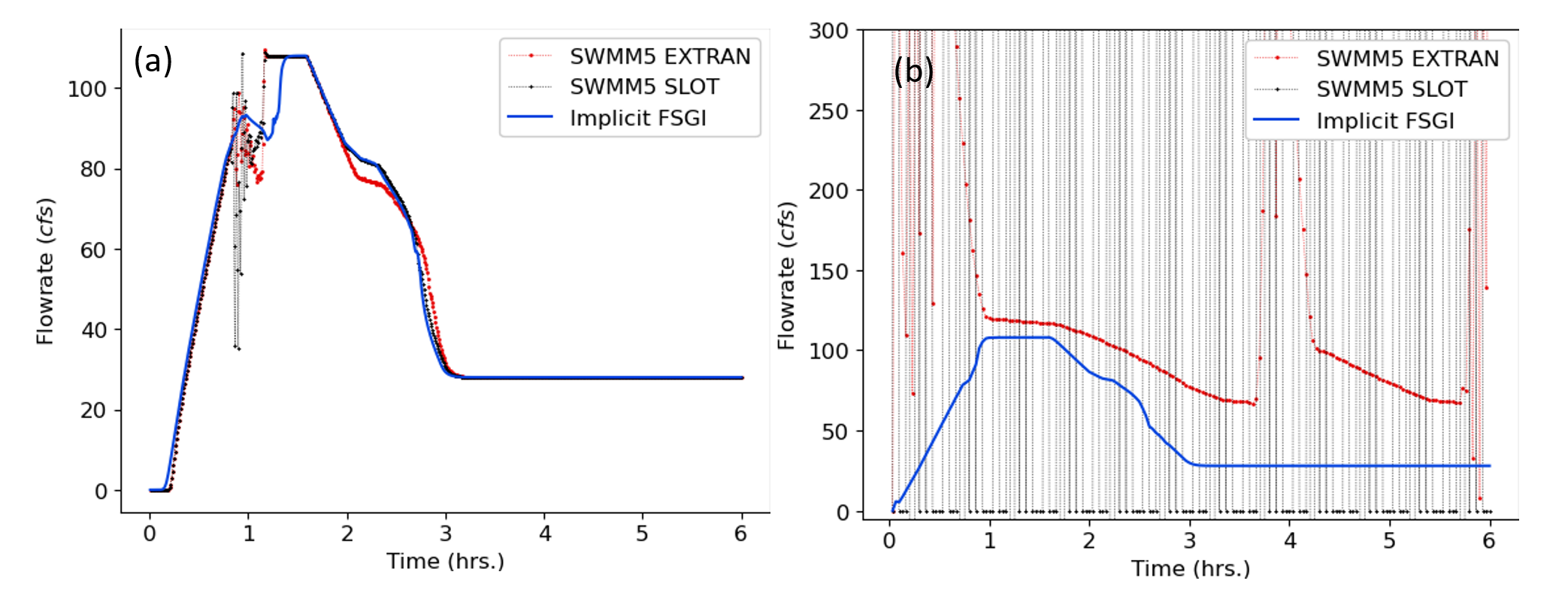
Figure 6: TEST 3 flowrate comparisons for link 105 between SWMM5 EXTRAN, SWMM5 SLOT and implicit FSGI for a routing timestep of (a) 5 seconds and (b) 120 seconds.
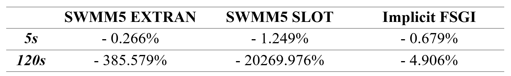
Figure 6 depicts the flowrate in link 105 for SWMM5 EXTRAN, SWMM5 SLOT and implicit FSGI for 5 second and 120 second routing time steps. For the 5 second routing time step, both SWMM5 EXTRAN and SLOT show signs of instability while the implicit FSGI is completely stable. For the 120 second routing time step, both SWMM5 EXTRAN and SLOT are unstable whereas the implicit FSGI is stable and conserves mass. The mass balance errors for both scenarios are shown in Table 3.
Table 3: TEST 3 mass balance error comparison
This test network is an inverted siphon and the profile is shown in Figure 7. All conduits are circular pipes 100-ft in length and 4-ft in diameter. The inflow hydrograph is a 3-hour square wave with 100 cfs magnitude. The simulation was carried out for a 5-hour duration using 5 second and 120 second routing time steps.
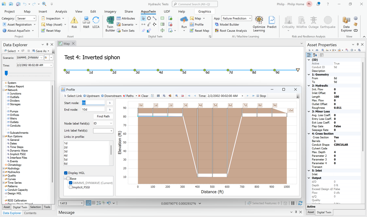
Figure 7: Profile view of TEST 4.
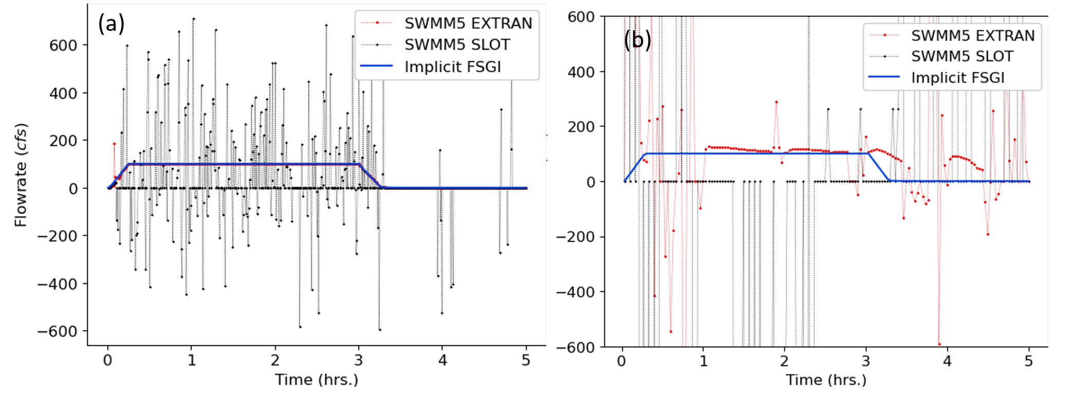
Figure 8: TEST 4 flowrate comparisons for link 5 between SWMM5 EXTRAN, SWMM5 SLOT and implicit FSGI for a routing timestep of (a) 5 seconds and (b) 120 seconds.
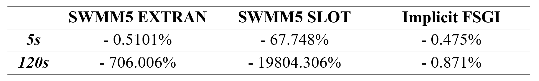
Figure 8 depicts the flowrate in link 5 for SWMM5 EXTRAN, SWMM5 SLOT and implicit FSGI for 5 second and 120 second routing time steps. For a 5 second routing time step, both SWMM5 SLOT and implicit FSGI are stable. However, SWMM5 SLOT is completely unstable. For a 120 second routing time step, both SWMM5 EXTRAN and SLOT are unstable whereas implicit FSGI is stable and conserves mass. The mass balance errors for both scenarios are shown in Table 4.
Table 4: TEST 4 mass balance error comparison
The final test network is a sequence of conduits, each of which has a 3-ft offset from the invert of its inlet node. Each conduit is 100-ft long, 4-foot diameter circular pipe at a 3% slope. The profile of this layout is shown in Figure 9. The simulation was carried out for a 12-hour duration using 5 second and 120 second routing time steps.
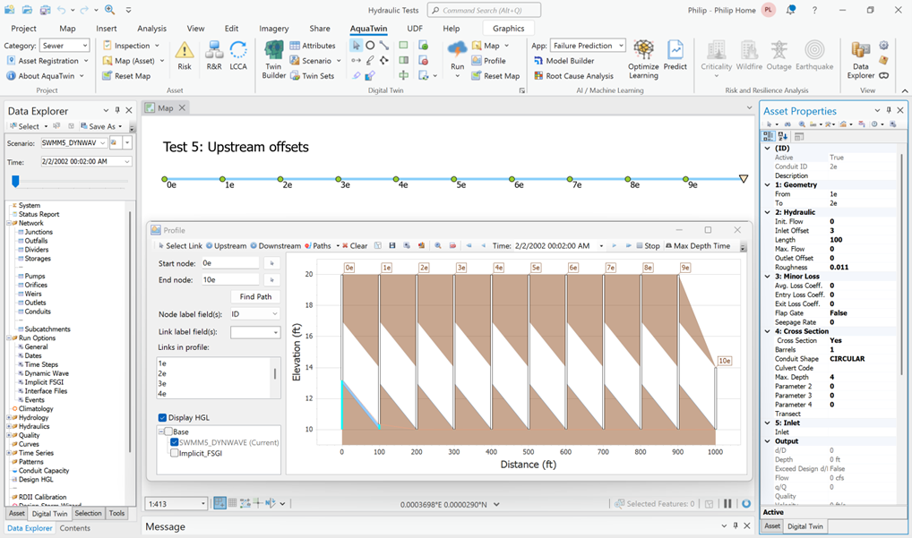
Figure 9: Profile view of TEST 5.
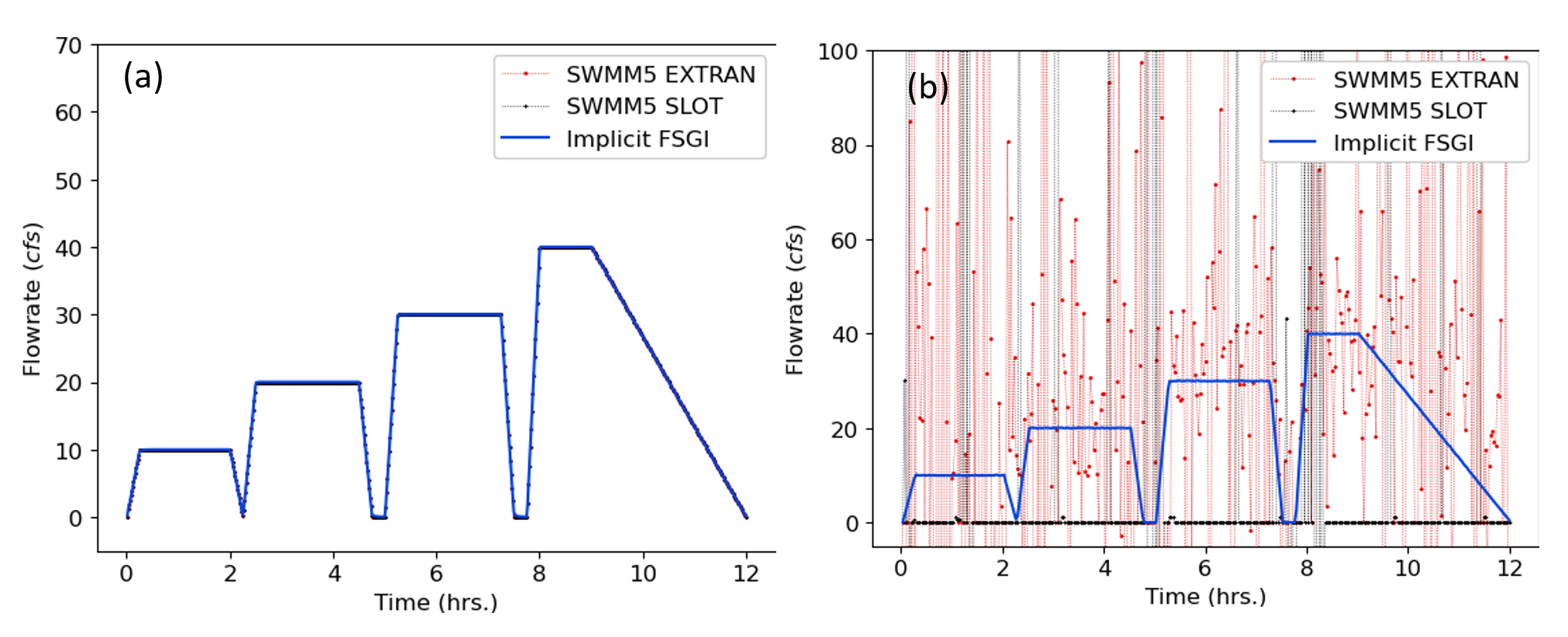
Figure 10: TEST 5 flowrate comparisons for link 1 between SWMM5 EXTRAN, SWMM5 SLOT and implicit FSGI for a routing timestep of (a) 5 seconds and (b) 120 seconds.
Figure 10 depicts the flowrate in link 1 for SWMM5 EXTRAN, SWMM5 SLOT and Implicit FSGI for 5 second and 120 second routing time steps. For the 5 second routing time step, SWMM5 EXTRAN, SLOT and implicit FSGI are stable. However, both SWMM5 EXTRAN and SLOT are unstable for a 120 second routing time step, whereas the implicit FSGI is stable and conserves mass. The mass balance errors for both scenarios are shown in Table 5.
Table 5: TEST 5 mass balance error comparison
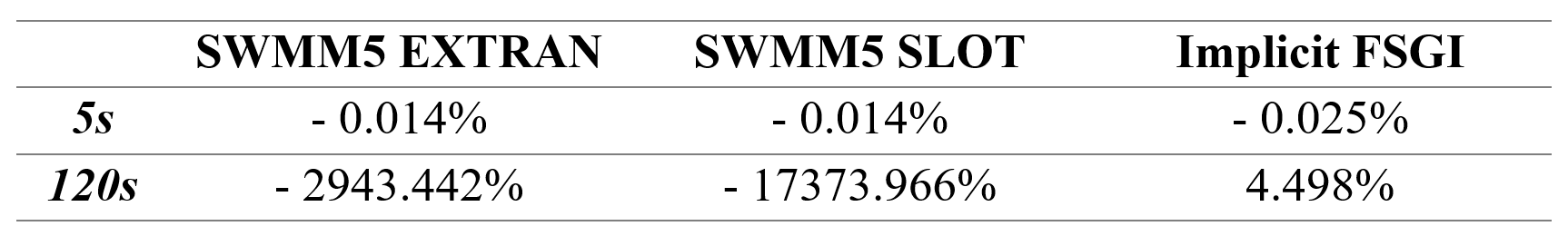
Figure 11: Network layout of the EXTRAN test cases.
We now analyze the nine EXTRAN test cases described in the SWMM5 QA/QC report (Rossman, 2006). Eight of the nine network layouts are shown in Figure 11. These EXTRAN test cases are simulated with 20 second and 900 second routing timesteps.
For the 20 second routing time step, SWMM5 EXTRAN, SLOT and implicit FSGI results are stable, and the mass balance errors are within an acceptable range. However, SWMM5 EXTRAN and SLOT are completely unstable for the 900 second routing time step while the implicit FSGI is stable and conserves mass. The 900 second routing time step simulation results for the EXTRAN test networks are shown in Figure 12 and the resulting mass balance error comparison is presented in Table 6.
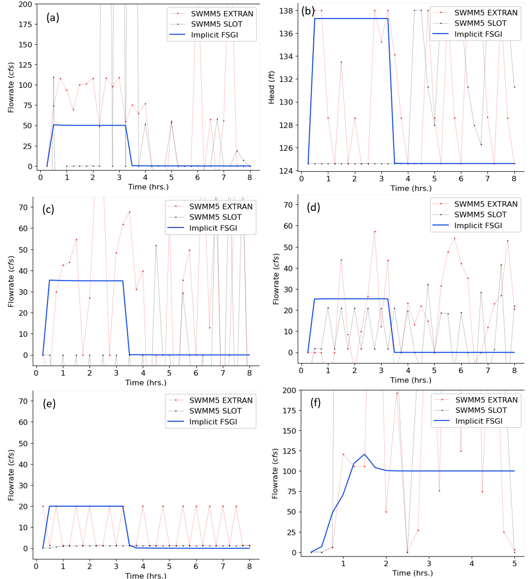
Figure 12: Selected results of the EXTRAN test networks for a 900 second routing timestep. (a) flowrate in conduit 8130 for EXTRAN 1, (b) head in junction 80408 for EXTRAN 2, (c) flowrate in weir 90010 for EXTRAN 3, (d) flowrate in orifice 90010 for EXTRAN 4, (e) flowrate in pump 90010 for EXTRAN 6, and (f) flowrate in conduit 10 in EXTRAN 9 networks.
Table 6: EXTRAN test networks mass balance error comparison
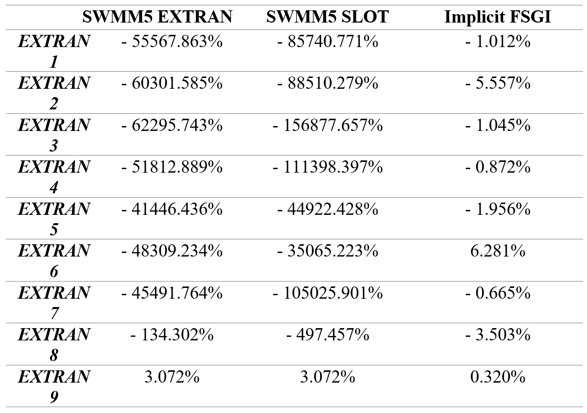
Figure 12 and Table 6 show that both SWMM5 EXTRAN and SLOT failed to simulate when the routing time step was 900 seconds. The implicit FSGI gave stable simulation results and effectively conserved mass for the nine EXTRAN networks even for a very large 900 second routing time step.
USER 1 network is shown in Figure 13 and consists of a 175-hectare drainage area divided into 58 subcatchments. The conveyance system contains 59 circular conduits connected to 59 junctions and a single outfall. The elevation profile of the main interceptor drops almost 19 m over 2.5 km. The hydraulic simulation was carried out using 5 second and 60 second flow routing time steps for a 7-hour duration with a 1-minute reporting time step.
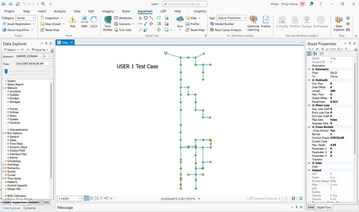
Figure 13: Network layout of the USER 1 test case.
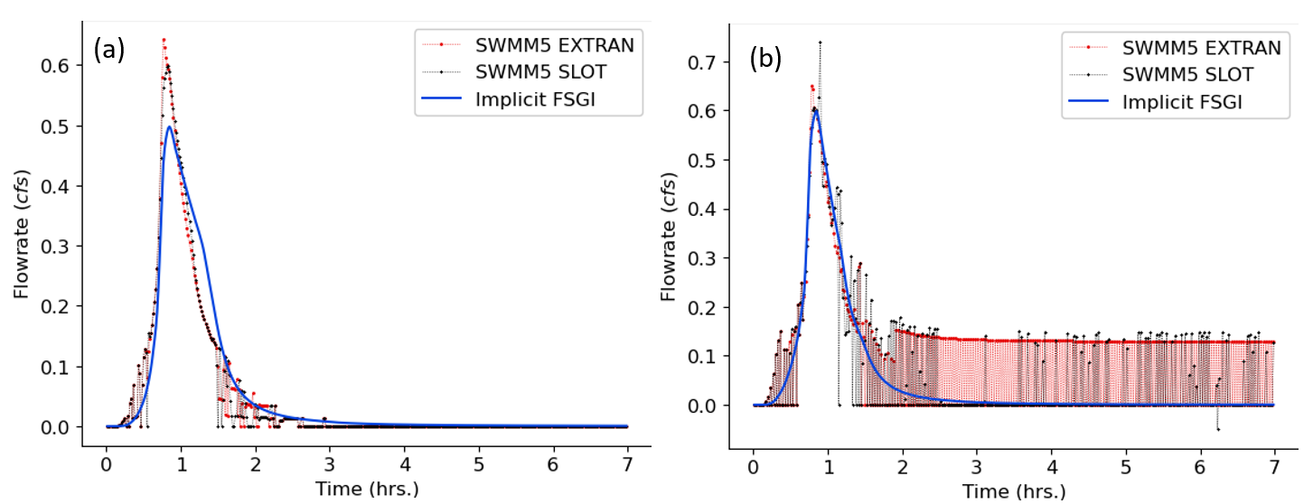
Figure 14: USER 1 flowrate comparisons for link 50 between SWMM5 EXTRAN, SWMM5 SLOT and implicit FSGI for a routing timestep of (a) 5 seconds and (b) 60 seconds.
Most of the links and nodes for the SWMM5 EXTRAN and SLOT solvers are stable for a 5 second routing step. However, signs of instability are seen in link 50. The implicit FSGI is completely stable at a 5 second routing step as depicted in Figure 14(a). For a 60 second routing time step, SWMM5 EXTRAN and SLOT are completely unstable whereas the implicit FSGI maintains unconditional stability as shown in Figure 14(b). The resulting mass balance error comparison for both scenarios is shown in Table 7.
Table 7: USER 1 mass balance error comparison
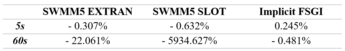
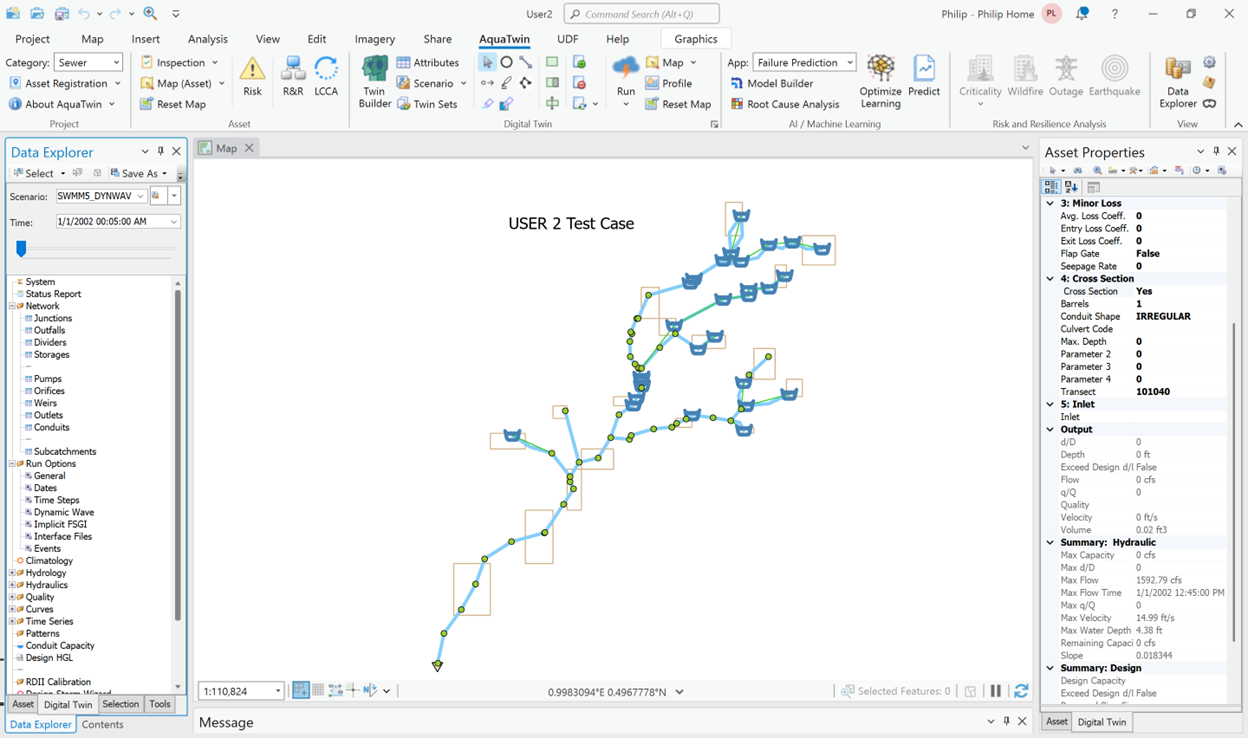
Figure 15: Network layout of the USER 2 test case.
The USER2 example network is shown in Figure 15 and consists of a 3.5 square mile drainage area broken into 17 subcatchments. The network is comprised of 83 conduits that are a mixture of irregular natural channels, open channels and closed pipes of various shapes. There are 28 storage units along with 19 weirs. Many of these storage units and weirs represent junctions with above-ground surface storage coupled with road overflows. A 4.4 inch, 24-hour design storm is applied to the network over a 36-hour simulation period using 5 second and 30 second flow routing time steps and a 5-minute reporting time step.
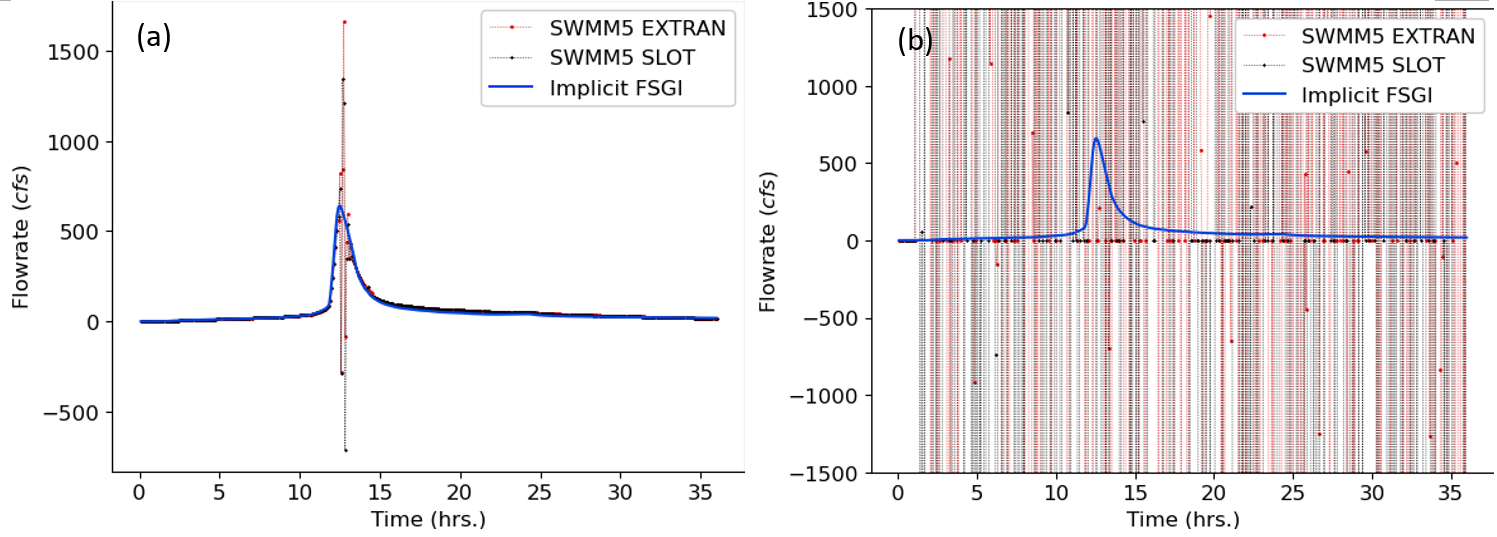
Figure 16: USER 2 flowrate comparisons for link TW01290between SWMM5 EXTRAN, SWMM5 SLOT and implicit FSGI for a routing timestep of (a) 5 seconds and (b) 30 seconds.
Both SWMM5 EXTRAN and SLOT show signs of instability in some of the links at a 5-second routing time step as depicted in Figure 16(a) while implicit FSGI is completely stable. At a 30 second routing time step, both SWMM5 EXTRAN and SWMM5 SLOT are completely unstable resulting in mass balance errors of -392380.397% and -121031.309%, respectively. The implicit FSGI is completely stable at a 30 second routing time step and the mass balance error is 2.225%.
The USER3 network is a combined sewer system comprising 168 subcatchments that encompasses an area of 6 square km. The network schematic is shown in Figure 17. The system contains 134 pipes of mostly circular or egg-shaped cross sections. Of the 141 nodes in the network, 6 are outfalls and 130 are manhole or catch basin structures that are represented as small storage units. There are 5 pumps in the network that discharge directly to the system’s outfalls. A 3-hour, 42 mm design storm was used in the simulation. This network was originally assessed using a 0.5 second routing step with a 1-minute reporting time step for a 6-hour total duration.
At a very small 0.5 second routing time-step, both SWMM5 EXTRAN and SWMM5 SLOT are stable resulting in mass balance errors of -0.023% and -0.106%, respectively. For the same routing time step, implicit FSGI is stable with an improved -0.009% mass balance error. At a large 120 second routing time step, the implicit FSGI remains stable with a mass balance error of -5.123%. However, SWMM5 EXTRAN and SLOT are completely unstable at the 120 second routing time step resulting in mass balance errors of -620.360% and -4219.874%, respectively. The effect of large routing time step on the stability of SWMM5 EXTRAN and SLOT is shown in Figure 18.
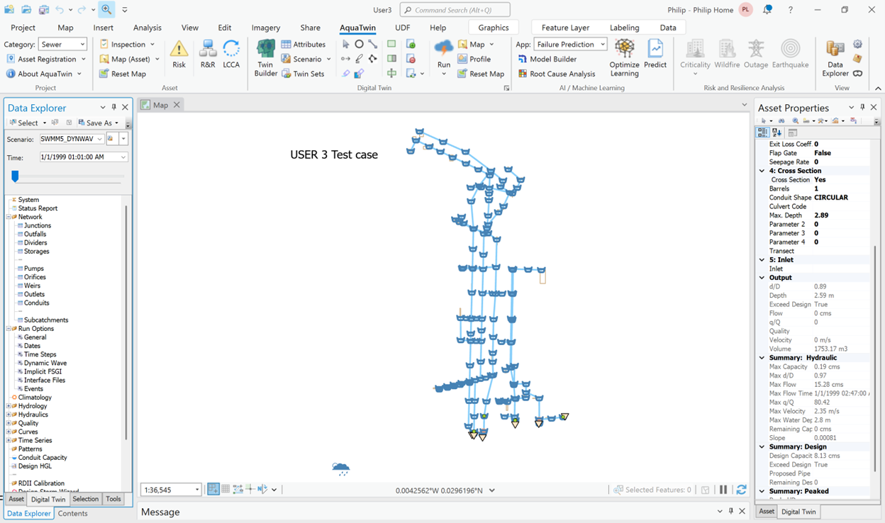
Figure 17: Network layout of the USER 3 test case.
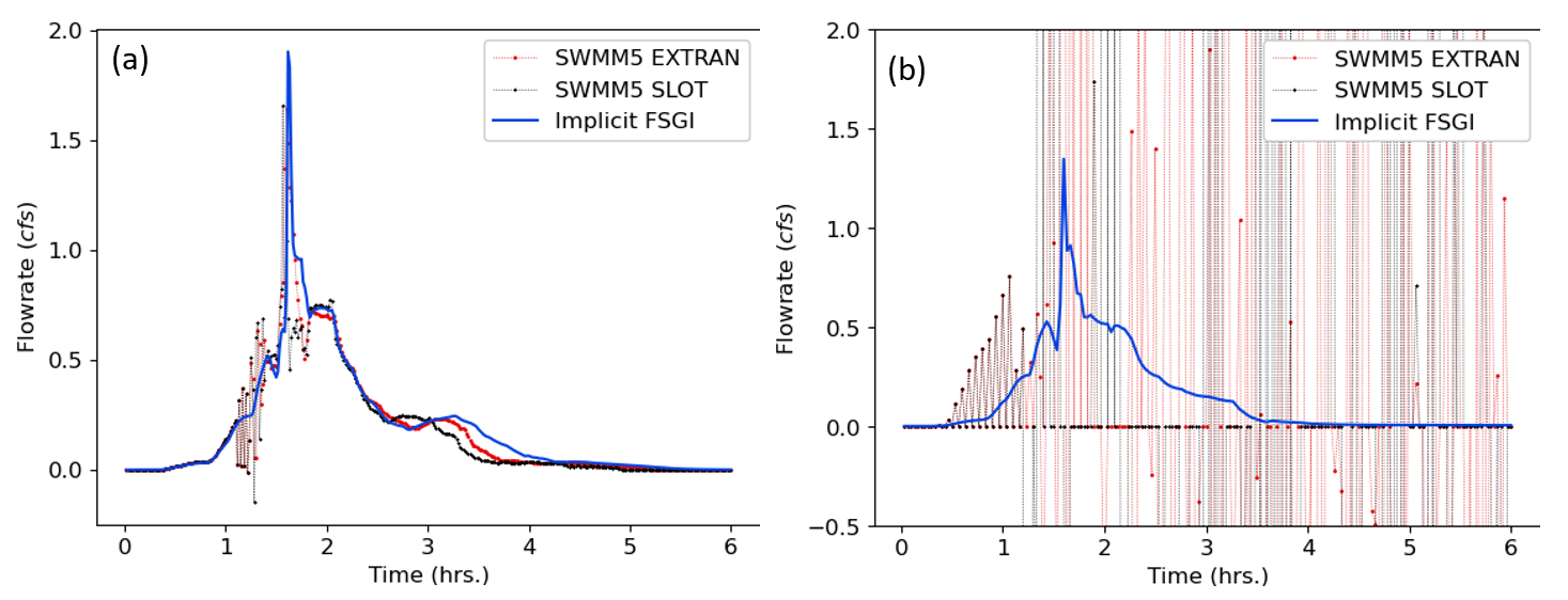
Figure 18: USER 3 flowrate comparisons for link CELCING between SWMM5 EXTRAN, SWMM5 SLOT and implicit FSGI for a routing timestep of (a) 0.5 seconds and (b) 120 seconds.
USER 4 network is a combined sewer system covering 528 acres divided into 112 subcatchments. The network schematic is shown in Figure 19. There are 209 circular conduits connecting 209 junctions and one outfall. Each subcatchment contributes both a dry weather sanitary flow (modeled as an external time series inflow applied to the subcatchment’s outlet node) as well as a wet weather flow produced for the storm. The system is analyzed over a 24-hour simulation period using 5 second and 15 second flow routing time steps with a 5-minute reporting time step.
With a 5 second routing time-step, both SWMM5 EXTRAN and SWMM5 SLOT are stable but result in mass balance errors of -6.459% and -10.576%, respectively. For the same 5 second routing time step, implicit FSGI is also stable with a much lower mass balance error of -0.004%. At a 15 second routing time step, both SWMM5 EXTRAN and SLOT are completely unstable with excessively high mass balance errors of -5052.202% and -75574.513%, respectively. In contrast, the implicit FSGI solution is stable at a 15 second routing time step with an excellent mass balance error of 0.490%. The effect of large routing time step on the stability of SWMM5 EXTRAN and SLOT is shown in Figure 20.
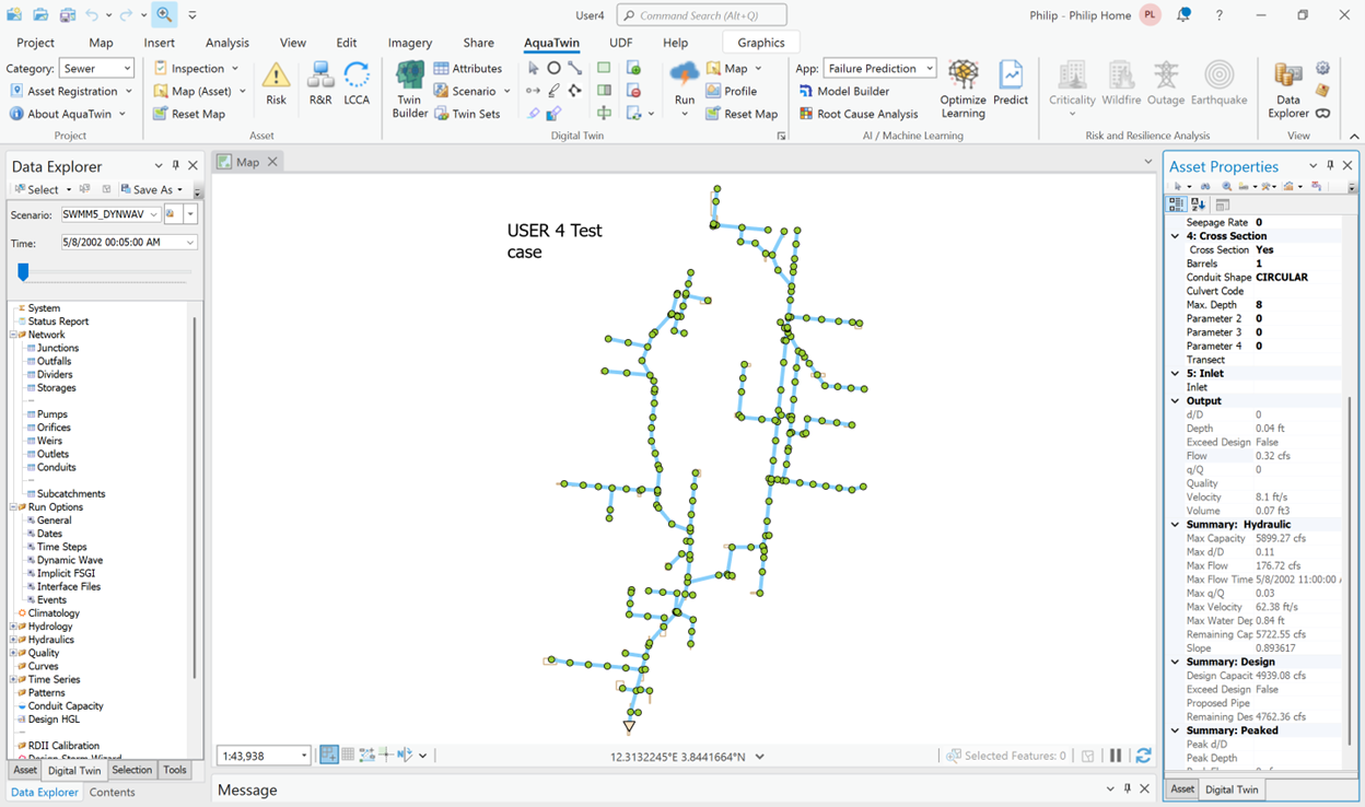
Figure 19: Network layout of the USER 4 test case.
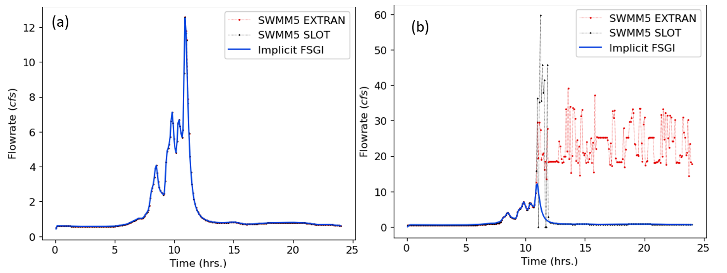
Figure 20: USER 4 flowrate comparisons for link 3701005-23701001 between SWMM5 EXTRAN, SWMM5 SLOT and implicit FSGI for a routing timestep of (a) 5 seconds and (b) 15 seconds.
The USER5 network represents a 1,177-acre watershed using 145 subcatchments draining to 273 conduits, the majority of which are irregular natural channels. The drainage system schematic is shown in Figure 21. A design storm event is routed through this network. In addition, the network receives inflows at 3 locations from upper portions of the watershed that are modeled separately. The network is analyzed over a 4-hour period using a 1-minute reporting time step and 0.5 second and 3 second flow routing time steps.
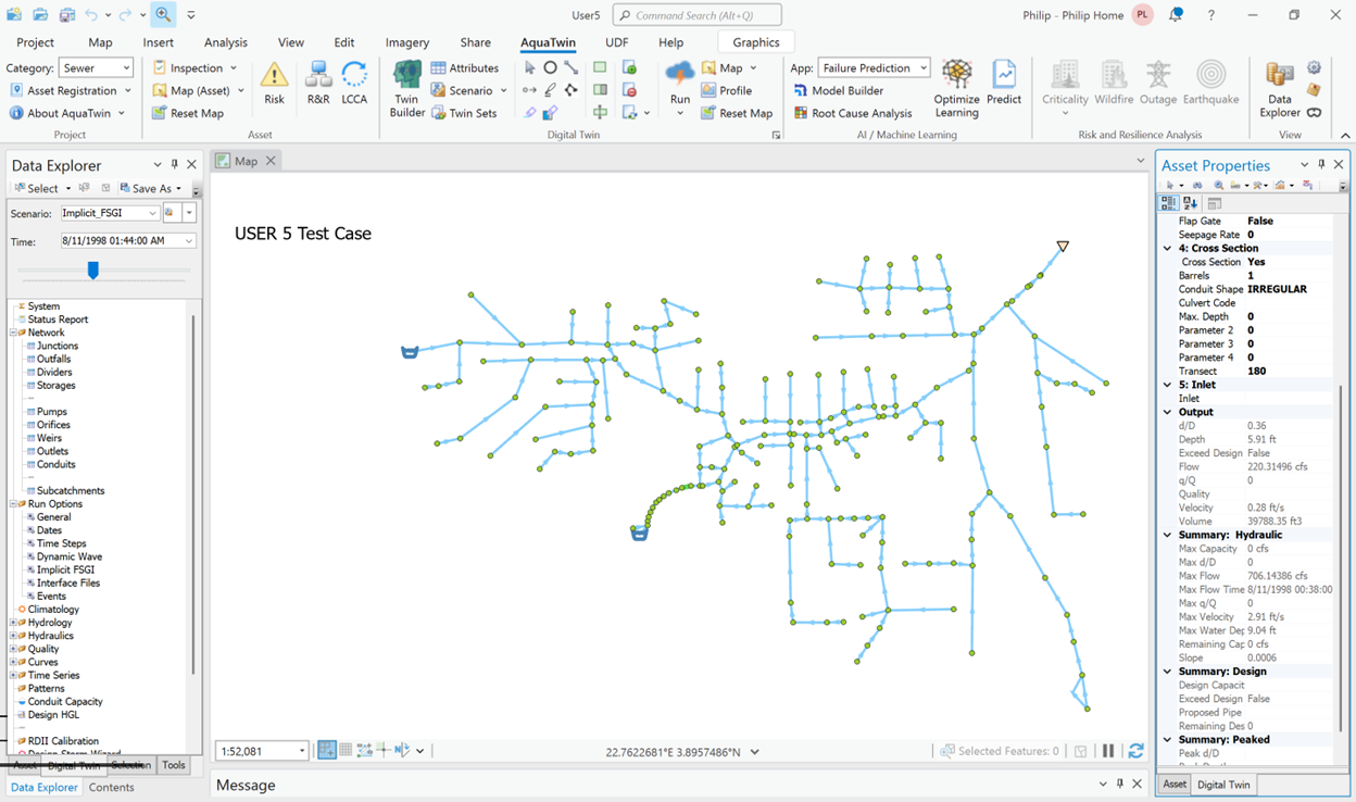
Figure 21: Network layout of the USER 5 test case.
At a 0.5 second routing time step, both SWMM5 EXTRAN and SWMM5 SLOT result in reasonable mass balance errors of -2.353% and -2.562%, respectively. However, model instability and huge flow oscillations are seen throughout the network despite the relatively small balance errors as depicted in Figure 22(a) and (b). With the same 0.5 second routing time step, implicit FSGI results in a stable simulation with a mass balance error of -1.898%. At a 3 second routing time step, both SWMM5 EXTRAN and SWMM5 SLOT exhibit significant instability and flow oscillations. However, the implicit FSGI produces stable and smooth results.
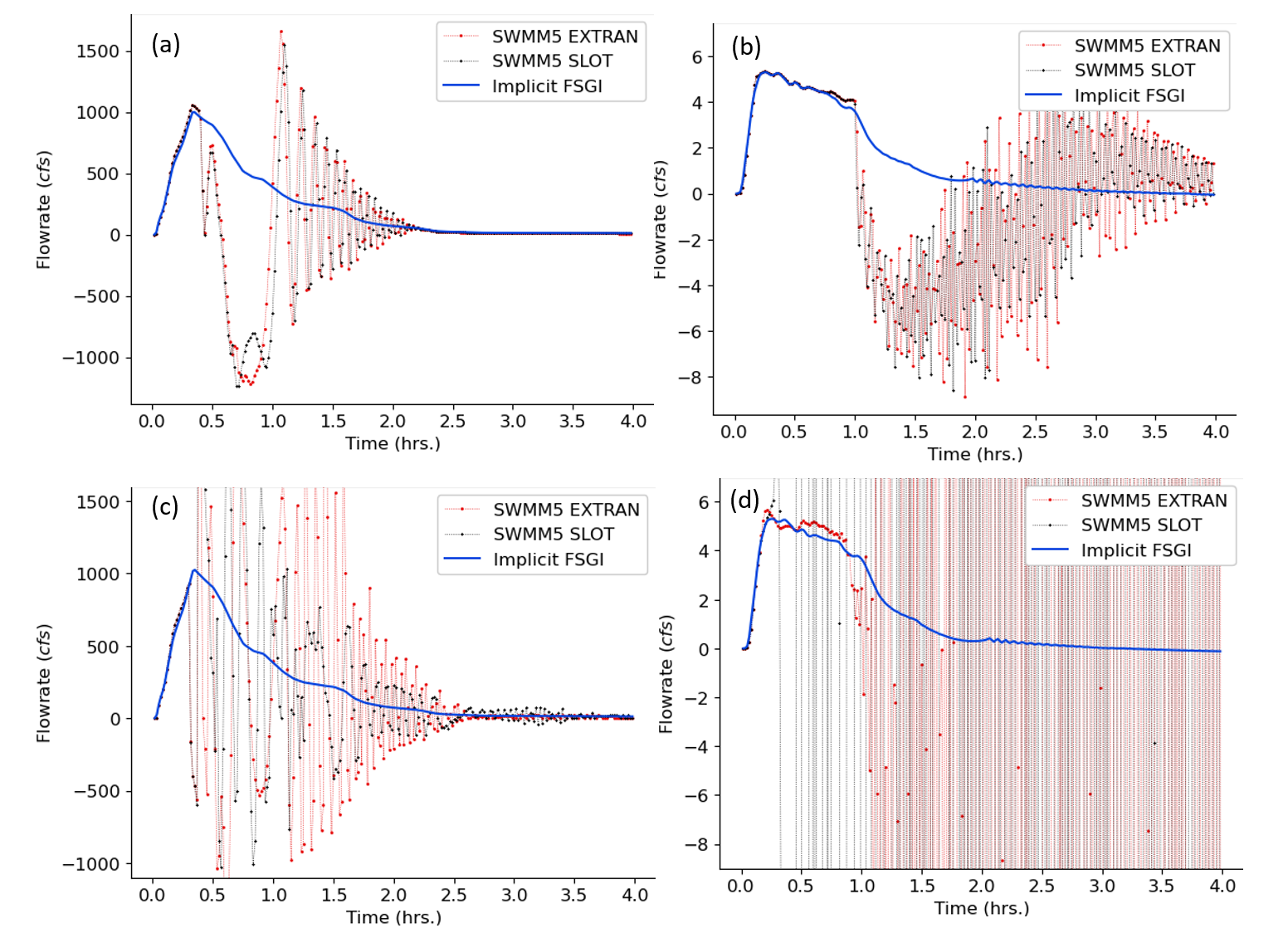
Figure 22: USER 5 flowrate comparisons for (a) link LIB_1 for a routing timestep of 0.5 second, (b) link 626 for a routing timestep of 0.5 second, (c) link LIB_1 for a routing timestep of 3 second, and (d) link 626 for a routing timestep of 3 second between SWMM5 EXTRAN, SWMM5 SLOT and implicit FSGI for a routing timestep of (a) 0.5 seconds and (b) 3 seconds.
Sewer Network_1 is a large and complex actual sewer network. It consists of 5818 conduits, 5637 junctions, 115 storage units, 31 pumps, 42 orifices, 101 weirs spread over 4375 subcatchments. In addition, this network has sophisticated pumps, weir and orifice controls. Engineering firm CDM Smith has provided this network for testing and this test case has been used here to benchmark the simulation run times between SWMM5 DYNWAVE (only SWMM5 EXTRAN surcharge model is used in this benchmarking since SWMM5 SLOT is completely unstable for this network) and implicit FSGI. The network was analyzed over a 12-hour simulation period with a 15-minute reporting time step.

Figure 23: Network layout of the Real Sewer Network_1 test case.
Using a 15 second variable routing time step, SWMM5 DYNWAVE simulation took 2 minute 11 seconds with a mass balance error of -1.337%. Implicit FSGI produced virtually identical results but with a larger 60 second fixed time step and a better mass balance error of 0.222 %. The resulting runtime of the implicit FSGI was 12 seconds, approximately 11 times faster than SWMM5 DYNWAVE and with better mass conservation.
Implicit FSGI presents a significant advancement in one-dimensional dynamic modeling of sewer/channel networks under both free surface and surcharged conditions. By embedding the flow equations within a system of implicit linear equations, FSGI significantly improves computational stability, speed and accuracy. The method’s novel use of recurrence relations substantially reduces the size of the solution matrix, leading to faster runtimes compared to traditional implicit schemes. Extensive validation and benchmarking against the industry-standard SWMM5 Dynamic Wave solver, using both QA/QC test cases and real-world sewer networks (only one actual sewer network was presented in this paper), reveal that the implicit FSGI outperforms SWMM5 DW not only in model stability and accuracy but also in faster run times. It is also important to note that, in some cases, SWMM5 DW can produce instability even when the associated continuity error is minimal. These results demonstrate that the implicit FSGI offers a more robust, efficient and reliable approach for modeling large and intricate sewer systems, making it an invaluable tool for hydraulic engineers and practitioners. Its computational advantages make it possible for applications of long-term simulation and real-time control for large sewer networks.
Courant, R., Friedrichs, K., & Lewy, H. (1928). Über die partiellen Differenzengleichungen der mathematischen Physik. Mathematische Annalen, 100(1), 32-74.
Lyn, D.A., & Goodwin, P. (1987). Stability of a General Preissmann Scheme. ASCE Journal of Hydraulic Engineering, 113(1), 16-28.
Meselhe, E.A. & Holly, F.M. (1997). Invalidity of Preissmann Scheme for Transcritical Flow. ASCE journal of Hydraulic Engineering, 123(7), 652-655.
Preissmann, A. (1961). Propagation des intumescences dans les canaux et les rivieres. First Congress of the French Association for Computation, Grenoble, 443-442.
Rossman, L.A. (2006). Storm Water Management Model, Quality Assurance Report: Dynamic Wave Flow Routing. Office of Research and Development, U.S. Environmental Protection Agency.
Rossman, L.A. (2017). Storm Water Management Model Reference Manual, Volume II – Hydraulics (EPA/600/R-17/111) [Technical Report]. Office of Research and Development, U.S. Environmental Protection Agency.