
AquaTwin Sewer 2D (AquaTwin) is a coupled 1D/2D urban drainage and flood modeling and mapping software developed by Aquanuity, Inc. (www.aquanuity.com) and built natively within the Esri ArcGIS Pro environment. It effectively simulates the dynamic exchange of flow between 1D pipe networks and 2D overland flow surfaces to accurately predict flood risks and network capacity. Its two-dimensional solver employs a conservative, finite-volume formulation of the two-dimensional shallow water equations (SWE). Seamless integration with ArcGIS Pro enables GIS-native model configuration, mesh generation, and results visualization, streamlining the workflow from raw data to actionable simulation results.
This report documents the application of AquaTwin to the benchmark test suite formalized by the UK Environment Agency (UK EA), a standard evaluation framework for 2D flood inundation software. Results from nine completed test cases are compared against 21 reference models that serve as the benchmark: the UK EA ensemble of 19 industry models (Néelz and Pender, 2013), HEC-RAS 2D (Brunner, 2018), and SRH-2D (Kramer, 2021). AquaTwin produces results consistent with established full-SWE solvers across tests spanning disconnected water body filling (Test 1), complex depression filling (Test 2), momentum conservation over a topographic obstruction (Test 3), flood wave propagation (Test 4), large-scale valley inundation (Test 5), multi-scale, laboratory-validated dam-break scenarios (Tests 6A and 6B), and urban runoff and drainage network surcharge modeling (Tests 8A and 8B).
Across the nine benchmark test cases, there are 83 unique test-point pairs reported. AquaTwin’s results are within the uncertainty defined by the reference models on 83 out of 83 test-points, and clustered within the central band of full-SWE solvers in the majority. Peak WSEs and flood arrival times tightly agree with HEC-RAS and SRH-2D to within the spread observed across the UK EA ensemble. Velocity magnitudes and time-series response signatures were similarly comparable.
These results demonstrate that AquaTwin is a rigorous and high-fidelity full-SWE simulation package whose performance is competitive with established industry tools while offering the practical advantages of a seamless GIS-integrated modeling environment. Thus, opening new avenues for solving urban stormwater and other flood risk management problems with unprecedented accuracy, stability, and speed.
Two-dimensional (2D) hydraulic models have become standard tools in flood risk management, infrastructure design, and urban drainage planning. As the number of available solvers has grown, so has the need for transparent, reproducible benchmarks that allow practitioners and regulators to evaluate model performance and flexibility on a consistent basis. This report applies that standard to AquaTwin Sewer 2D (AquaTwin), situating it within the established benchmark record and providing the evidentiary foundation that practitioners require when selecting flood modeling software.
Each test case is fully specified by Néelz and Pender (2013) and supported by files available in the UK public data repository (2D benchmarking: evaluating the latest generation of the hydraulic models for FCRM – GOV.UK), including topography, 2D domain geometry, initial and boundary conditions, sampling point locations, and required simulation duration and output resolution. This high degree of specification minimizes modeler discretion, ensuring that results are directly comparable across software packages and reproducible by third parties.
To provide context for the AquaTwin results, this report reproduces figures from previously published benchmark datasets. The primary source is the most recent report, Federal Highway Administration (FHWA) report Benchmarking of SRH-2D (Kramer, 2021; FHWA-RC-21-0006), which itself reproduced selected figures from two earlier reports: a U.S. Army Corps of Engineers (USACE) benchmarking study of HEC-RAS (Brunner, 2018; RD-51) and the original United Kingdom Environment Agency (UK EA) benchmarking study (Néelz and Pender, 2013; SC120002).
As a result, each test case result is presented as a quadruplicate figure (example, see Figure 1), with subfigures arranged as follows:
The UK EA “Ensemble” subfigure contains results from a composite of industry models that participated in the original study, including: InfoWorks 2D, MIKE FLOOD, TUFLOW, ANUGA, ISIS2D, SOBEK, and others. The HEC-RAS subfigure contains results from simulations run with HEC-RAS 2D full shallow water equations (FEQ) and diffusion wave (Diff Wav) solvers.
HEC-RAS and SRH-2D were selected as comparators for two reasons: both are widely used in the U.S. for simulations that require regulatory approval, and both have published benchmark results for the full UK EA test suite, against which AquaTwin results can be directly compared. The UK EA Ensemble is retained as a reference for the broader spread of SWE solver behavior.
Rather than attempting to digitize the results from each reference report, herein the AquaTwin results are compared by highlighting key markers, including wave arrival timing, peak magnitude and timing, and overall profile shape, between each results subfigure.
Due to subfigures being replicated from previous reports, the aspect ratios and axis-limits may not be exactly aligned. Readers should take care to identify key time-series transitions (e.g., wave arrival times, peak timing and magnitude) when comparing across reports. Where possible, the AquaTwin results were formatted to align visually with the UK EA Ensemble.

Figure 1. Test Case 3 – Point 5 WSE. Top left: AquaTwin (this study). Top right: Ensemble, reproduced from Néelz and Pender (2013); as it appears in Kramer (2021), p. 3-13. Bottom left: HEC-RAS, reproduced from Brunner (2018); as it appears in Kramer (2021), p. 3-13. Bottom right: SRH-2D, reproduced from Kramer (2021), p. 3-13.
The 2D SWEs simplify the more general Reynold’s-averaged Navier-Stokes equations by assuming hydrostatic pressure, depth-averaged velocities, small bed slopes, and quasi-steady friction. Additionally, turbulence and viscosity are typically neglected.
The resulting governing equations for the 2D SWEs can be written in the form:
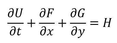
where U encodes the mass and momentum per unit area (i.e., water depth and depth-averaged velocity), F and G describe the flux of those quantities through cell faces in the x and y directions (due to convective acceleration and pressure gradients), and H is the forcing function (i.e., difference between bed slope and friction slope).
The 2D SWEs are primarily used for modeling situations where the horizontal length scales of the flow (i.e., in the x- and y-directions) are much greater than the characteristic flow depth and the pressure distribution is effectively hydrostatic (i.e., gradually varied flow). For example, floodplain inundation and overland flow routing are common applications of the 2D SWEs (Vreugdenhil, 1994)
The benchmark tests used in this study were originally formalized by Heriot & Watt University to support an open call for 2D flood inundation modeling software by the United Kingdom Environment Agency (UK EA) in 2009. Modeling software vendors voluntarily participated in the study; Néelz & Pender (2013) finalized the ensemble report.
Subsequently, the UK EA benchmark test case suite has been adopted as a standard evaluation framework for 2D flood inundation modeling software, including by Brunner (2019, HEC-RAS) and Kramer (2021, SRH-2D). Together, the test cases span the range of physical regimes encountered in practical flood risk modeling, from low-momentum fill-dominated inundations (Tests 1-2) to momentum-critical, rapidly varying flow (Tests 3, 5, 6) to urban drainage coupling (Tests 8A-8B), providing a comprehensive basis for evaluating solver capability.
Typically, the benchmark results from the reference models on the UK EA test cases included water surface elevations (WSE) and magnitudes of velocity (velocity) at specified points in the simulation domain. For some test cases, cross-section profiles of maximum WSE or other time series data were required.
HEC-RAS 2D is developed and maintained by the U.S. Army Corps of Engineers Hydrologic Engineering Center and is among the most widely used 2D hydraulic solvers in the U.S. federal flood risk practice (Brunner, 2021). SRH-2D is developed by the U.S. Bureau of Reclamation and adopted by the Federal Highway Administration for bridge hydraulics and roadway inundation analysis (Lai, 2008). Both solvers implement the full shallow water equations, and both have published independent benchmark results against the UK EA test cases – Brunner (2018, Report RD-51) for HEC-RAS and Kramer (2021, Report FHWA-RC-21-0006) for SRH-2D, respectively.
The ensemble report from Néelz & Pender (2013) presented 19 software packages covering a wide spectrum of numerical approaches to solving the 2D SWEs. The various software packages can be categorized based on how many terms of the SWEs each model retains.
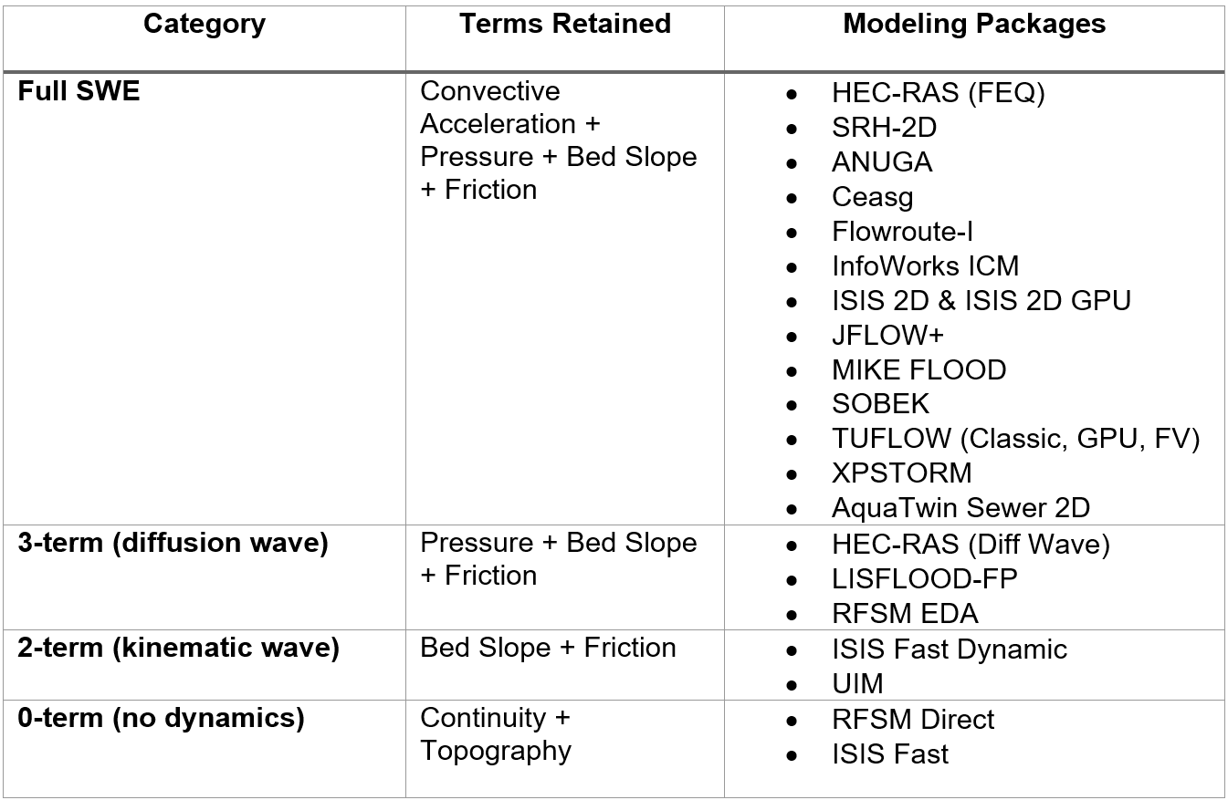
Table 1. Comparison models from Neelz & Pender (2013), Brunner (2018), and Kramer (2021), organized by SWE terms retained. Amended to include AquaTwin Sewer 2D.
Not every reference model was appropriate for all Test Cases. For example, some of the lower-term models were neglected for momentum-based simulations, HEC-RAS was neglected for the super high-resolution dam-break scenario, and SRH-2D was neglected for coupled hydraulic-hydrologic modeling. Similarly, AquaTwin was not exercised on Test Case 7 from the UK EA report – linking river channel and overbank flow.
Wherever possible, all reported data from the three reference reports were included.
AquaTwin falls within the full-SWE category of solvers. More specifically, AquaTwin employs a conservative, finite-volume solver formulation capable of shock capturing – the resolution of discontinuities in the solution to Eq. 1 that arise where the flow regime changes abruptly, as in hydraulic jumps and dam-break fronts. This finite‑volume, shock‑capturing approach is shared by several benchmark participants and differs from the finite‑difference formulations used by others; it is especially well suited to the transcritical and rapidly varied flows exercised by Tests 3, 5, 6A & 6B. The AquaTwin engine operates on an unstructured triangular mesh where the cell-averaged elevation is imputed from a digital elevation model (DEM) raster.
The simulation results from AquaTwin presented herein were obtained using AquaTwin v5.1.5 (released on May 26, 2026). For more information about flood modeling with AquaTwin visit https://aquanuity.com/products/aquatwin-sewer-2d/.
The UK EA benchmark test cases were configured within AquaTwin’s ArcGIS Pro-based modeling environment (shown in Figure 2). The domain boundary, DEM, and sample point locations were imported from the test case supporting files directly into AquaTwin as ArcGIS feature classes, which streamlines the workflow from raw data into a ready-to-run simulation. Time-varying boundary conditions, roughness parameters, and structure mesh resolution were also specified in the test case instructions and imported into the model through AquaTwin’s 2D Modeling wizard.
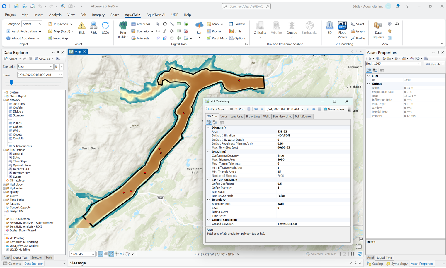
Figure 2. Screenshot of Test Case 5 within AquaTwin’s ArcGIS Pro Interface. The DEM, 2D Area boundary, inflow location, and sample points are shown, along with simulation parameters in the 2D modeling wizard.
Simulation results are visualized through the AquaTwin Sewer 2D – Flood Viewer, a dedicated 3D rendering environment that displays flood depth and velocity outputs against a DEM-based terrain surface (Figure 3). The terrain is rendered with configurable vertical exaggeration, hillshade, and basemap integration, enabling results to be interpreted directly in the geospatial context. Flood depths are displayed using a customized color symbology mapped to water depth; in Figure 3 warm colors (yellow-red) indicating greater depths and cool colors (blue-green) indicating shallower inundation. In addition to depth visualization, the Flood Viewer supports animated particle tracers that render instantaneous velocity vectors across the 2D domain, providing an intuitive representation of flow direction and speed at each timestep. A “Worst Case” summary mode computes and displays the maximum depth recorded at each cell across all timesteps, useful for rapid identification of peak inundation extents. Graph and Section tools allow the user to view and export time series of depth and velocity at individual points and along cross-sections. Together, these visualization tools support both internal analysis and stakeholder communication of simulation results.
Wherever possible, visualizations from the AquaTwin Sewer 2D – Flood Viewer were included to provide context and aid interpretation of the test case time series results.

Figure 3. Screenshot of Test Case 5 visualized with the AquaTwin Sewer 2D – Flood Viewer. The DEM “terrain” is exaggerated by 2.0x, with hillshading to emphasize vertical relief. The “Worst Case” flood depth is symbolized with a blue-yellow-red heatmap.
The domain is an initially dry rectangular grid (700 m x 100 m) of adversely sloping topography with a small internal depression (Figure 1.1). A time-varying level boundary condition (Figure 1.2) at the downhill end creates an elevation gradient that drives water up the channel and over the hill to the depression. The height is maintained for some time to allow the water to stabilize, before dropping and draining the downslope, leaving some water in the depression. All other boundaries are walls. This simple test is designed to simulate tidal conditions and challenge each solver’s wetting/drying front mechanics and mass conservation.

Figure 1.1 Profile of channel.
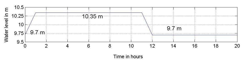
Figure 1.2 Time-varying boundary condition.
Points 1 and 2 are located at stations 400 m and 600 m, respectively, in Figure 1.1. Model outputs were reported every 60 s for the 20-hour simulation time.
The DEM (from the UK EA reference documents) was imported into a new AquaTwin project. The 2D boundary was initialized as a 700 m x 100 m rectangular polygon. The default roughness was specified to be 0.03 and there was no infiltration. Grid resolution (~700 nodes) was recommended by the test.

Figure 1.3 AquaTwin modeling parameters and interface. Selected mesh elements reflect Points 1 and 2.

Figure 1.4 AquaTwin Sewer 2D – Flood Viewer 3D rendering of water level boundary and flow condition at t = 84 min simulation time.

Figure 1.5. Point 1 WSE. Top left: AquaTwin. Top right: Ensemble, reproduced from Néelz and Pender (2013); as it appears in Kramer (2021), p. 2-4. Bottom left: HEC-RAS, reproduced from Brunner (2018); as it appears in Kramer (2021), p. 2-4. Bottom right: SRH-2D, reproduced from Kramer (2021), p. 2-4.
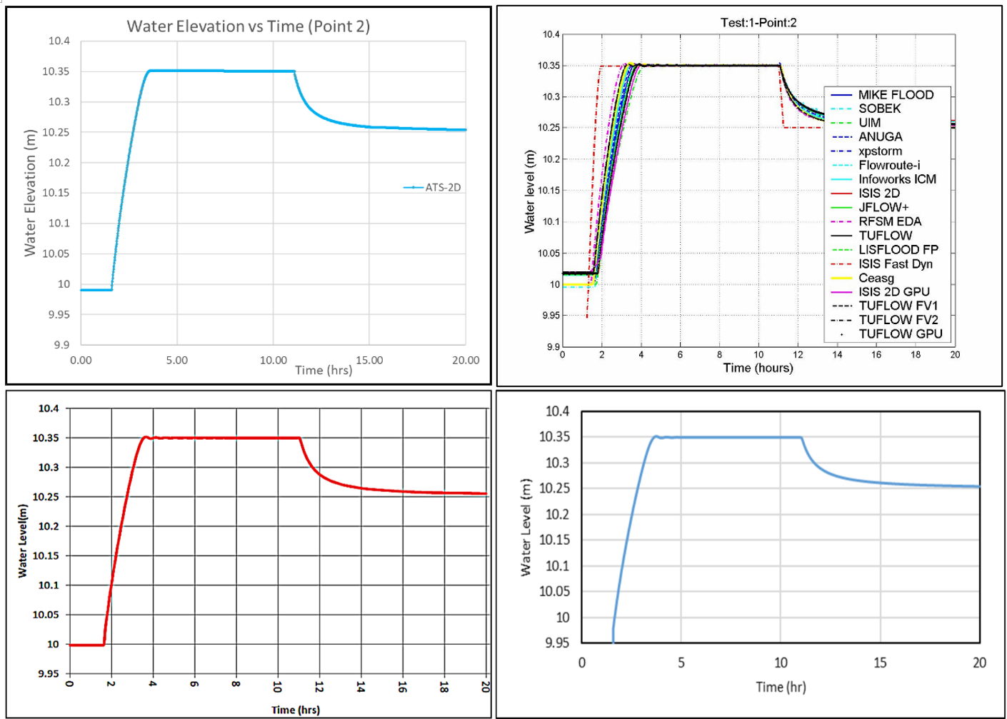
Figure 1.6. Point 2 WSE. Top left: AquaTwin. Top right: Ensemble, reproduced from Néelz and Pender (2013); as it appears in Kramer (2021), p. 2-5. Bottom left: HEC-RAS, reproduced from Brunner (2018); as it appears in Kramer (2021), p. 2-5. Bottom right: SRH-2D, reproduced from Kramer (2021), p. 2-5.
Both Point 1 and Point 2 are within the small depression on the other side of the internal hill from the boundary condition, and both start with an initially dry condition such that the elevation at t = 0 hrs is equivalent to the ground elevation at those points.
During the simulation, AquaTwin reproduces the reference behavior at both points essentially exactly; water levels rise from the initial dry-bed condition beginning at t = 1.0-1.5 hrs following the boundary condition ramp, further increase to the 10.35 m plateau by t = 3.5hrs, and recede back to the elevation of the internal hill by t = 20 hrs. The peak values and endpoint values (10.35 m and 10.25 m) match the expected outcomes from the Ensemble. The AquaTwin curve timing is also indistinguishable from both HEC-RAS and SRH-2D reference curves at both points.
Test Case 1 is fundamentally a mass-conservation and wetting/drying front sanity check. AquaTwin’s strong performance here should be interpreted as confirmation of basic mass-conservation and flow-routing mechanics.
Test Case 2 evaluates low-momentum, fill-dominated inundation over complex topography – the same physical regime as Test Case 1, but over a full 2D floodplain, rather than a single channel. The domain (Figure 2.1) is a 2000 m x 2000 m floodplain containing a 4 x 4 array of shallow depressions, each roughly 0.5 m deep with smooth, sinusoidal side slopes. The underlying DEM is constructed as the product of two sinusoidal functions, one oriented north-south and one east west, superimposed on a gentle regional slope (1:1500 north-south and 1:3000 west-east). Together, these functions produce a net elevation drop of approximately 2m from the northwest to the southeast corner.
Inflow enters along a 100 m segment along the northernmost edge of the west boundary, specified as a trapezoidal hydrograph peaking at 20 m3/s with a base time of approximately 85 minutes (Figure 2.2). All other domain boundaries are walls (i.e., no flow) and the domain is initially dry. The simulation runs for 48 hours to allow inundation to stabilize, with reporting time suggested as every 5 minutes for the sampling points at the center of each depression (Figure 2.1).
A uniform Manning’s roughness of n = 0.003 is applied across the domain; no infiltration is permitted. The resolution is specified that the domain is composed of ~10,000 computational elements.

Figure 2.1. Schematic of the 2D domain with sinusoidal depression elevations (0.1 m contours). Sampling point numbering convention and inflow boundary condition are shown.

Figure 2.2. Screenshot of inflow boundary condition constructed in AquaTwin.
The DEM (from the UK EA reference documents) was imported into a new AquaTwin project. The 2D boundary was initialized as a 2000 m square starting at the origin (Figure 2.1). The inflow boundary condition hydrograph (Figure 2.2) was implemented at the northwest corner; a guide polyline layer was added with lines every 500 m to identify each depression sampling point (Figure 2.3).
The meshing settings were calibrated such that the total number of computational elements was ~10,000. Horton’s infiltration model was modified such that there was no infiltration. The simulation was run at a 1 s time step for 48 hours of runtime with results output every 30 seconds.

Figure 2.3. Screenshot of the Test Case 2 domain with grey-scale DEM, pink 2D boundary, red sample point guidelines, and orange inflow boundary condition shown. Also visible is the 2D Modeling wizard with runtime options.
Figure 2.4 shows an illustration from the AquaTwin Sewer 2D – Flood Viewer at an intermediate simulation time depicting the inflow condition and the already filled depressions containing Points 4, 8, and 3, along with the spreading of the flood wave to subsequent depressions in the southeast direction.
Of the 16 total sampling points for Test Case 2, only 11 receive water due to the limited duration of the inflow boundary condition. For concision, only Points 4, 7, and 10 (wetted points on the diagonal) are shown herein. WSE timeseries for the remaining sampling points can be found in Appendix A.2.

Figure 2.4. Screenshot from AquaTwin Sewer 2D – Flood Viewer at t = 2hrs. Warm colors (i.e., yellow-red) indicate deeper water depths; cool colors (i.e., blue-green) indicate shallow water.
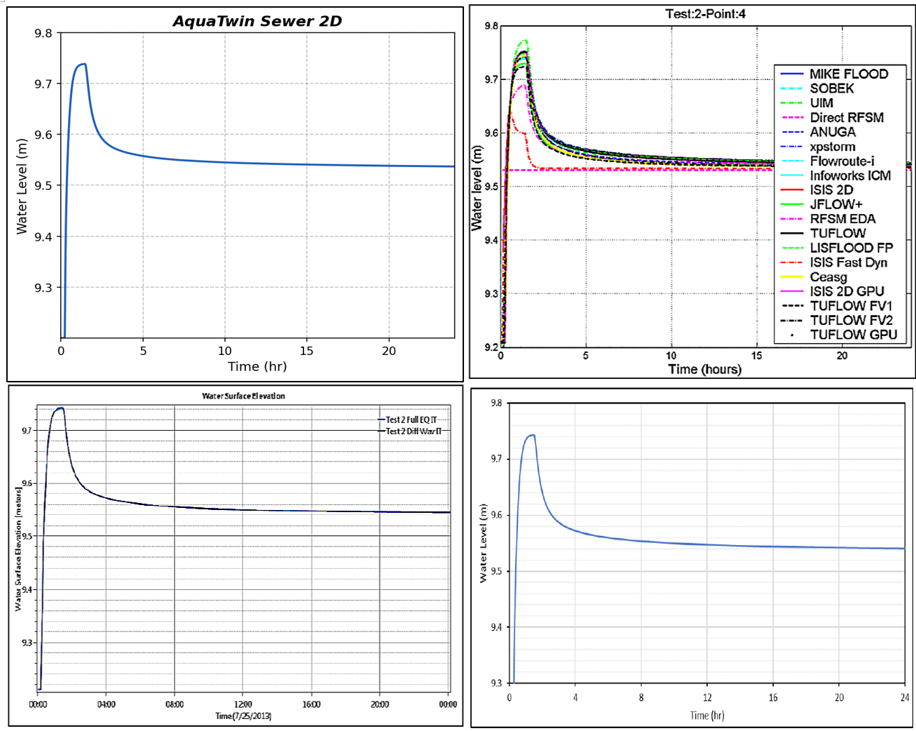
Figure 2.5. Point 4 WSE. Top left: AquaTwin. Top right: Ensemble, reproduced from Néelz and Pender (2013); as it appears in Kramer (2021), p. 3-6. Bottom left: HEC-RAS, reproduced from Brunner (2018); as it appears in Kramer (2021), p. 3-6. Bottom right: SRH-2D, reproduced from Kramer (2021), p. 3-6.
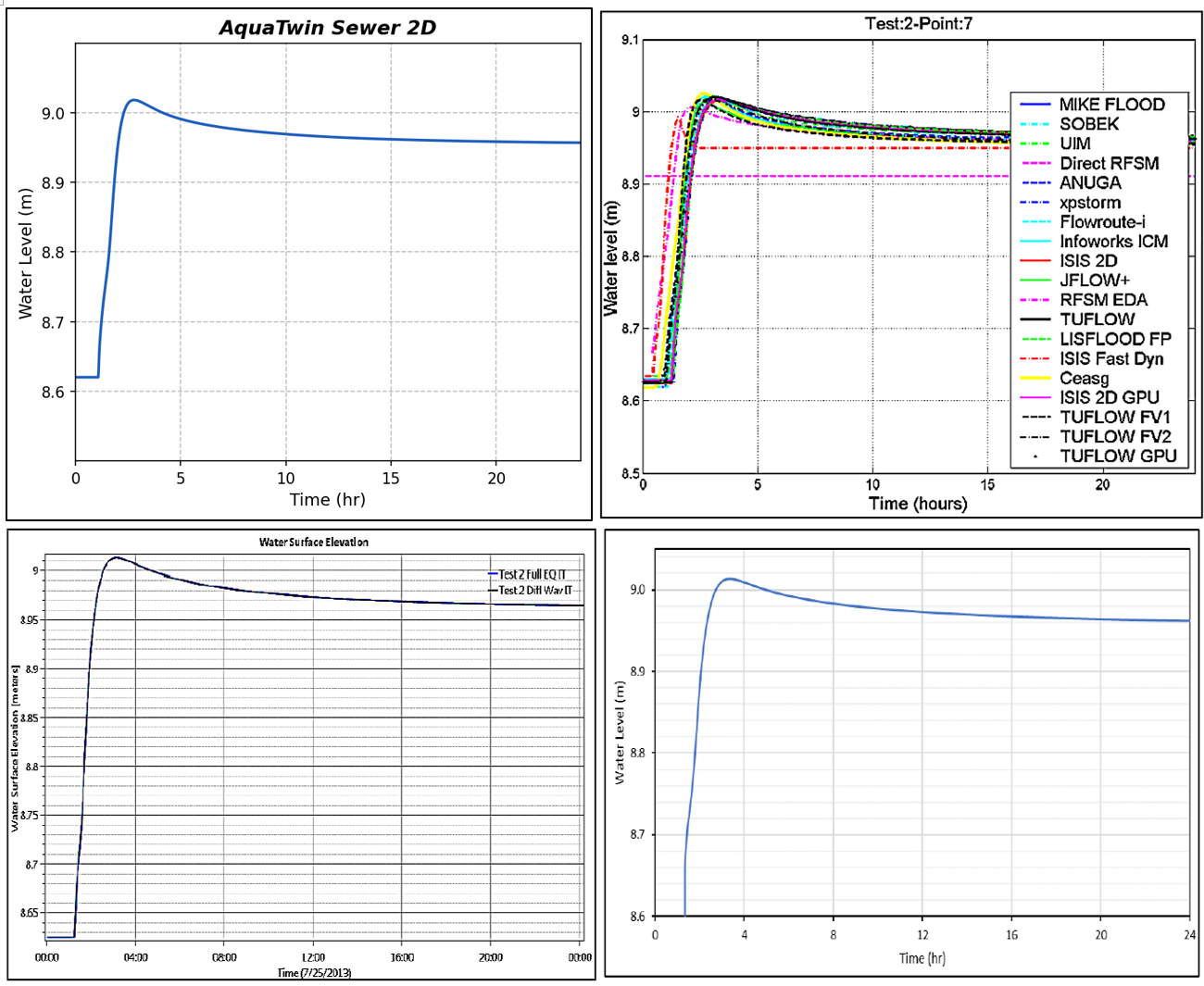
Figure 2.6. Point 7 WSE. Top left: AquaTwin. Top right: Ensemble, reproduced from Néelz and Pender (2013); as it appears in Kramer (2021), p. 3-11. Bottom left: HEC-RAS, reproduced from Brunner (2018); as it appears in Kramer (2021), p. 3-11. Bottom right: SRH-2D, reproduced from Kramer (2021), p. 3-11.
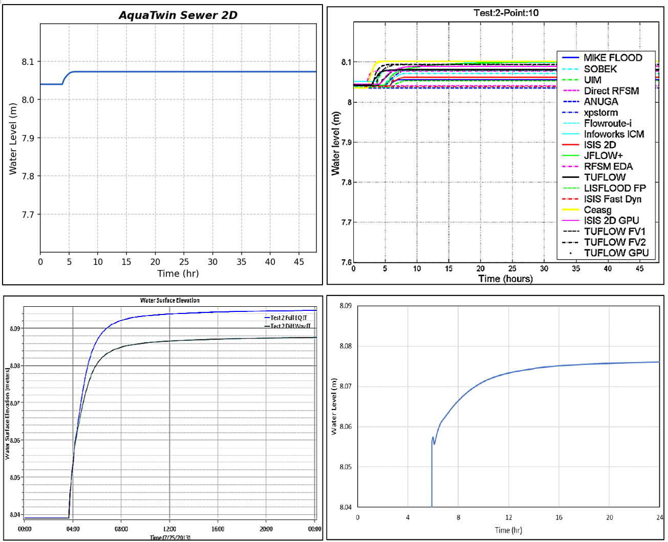
Figure 2.7. Point 10 WSE. Top left: AquaTwin. Top right: Ensemble, reproduced from Néelz and Pender (2013); as it appears in Kramer (2021), p. 3-16. Bottom left: HEC-RAS, reproduced from Brunner (2018); as it appears in Kramer (2021), p. 3-16. Bottom right: SRH-2D, reproduced from Kramer (2021), p. 3-16.
Points 4, 7, and 10 lie along the NW–SE diagonal at increasing distance from the inflow, and the results reflect that progression. AquaTwin predicts a peak of 9.74 m at approximately t = 1:20 at Point 4 (nearest the inflow). Further afield at Point 7, the flood wave arrival occurred at t = 1:05 and the peak WSE reached 9.0 m at t = 2:50. Lastly, the wave arrival was delayed until t = 3:50 at Point 10, where the water level plateaued at 8.07 m rather than producing a distinct peak. Timing and magnitude at all three points track most closely with TUFLOW, HEC-RAS (Full EQ), and SRH-2D (a.k.a., other full-SWE solvers in the comparison set).
The UK EA Ensemble spread is noticeably wider here than in Test Case 1, particularly in arrival and peak timing, and HEC-RAS’s Full EQ and Diffusive Wave solutions diverge visibly at Point 10. Both point to some residual momentum sensitivity in this test, despite Test 2 being designed primarily as a low-momentum fill test.
Test Case 3 simulates a brief flood pulse flowing down an initially dry rectangular channel towards a small internal hill (Figure 3.1). While the volume of the time-varying inflow (Figure 3.2) is just enough to fill the depression centered at X = 150m, some flow is expected to overtop the depression due to momentum conservation and setting in the depression centered at X = 250m. This test case assesses the solvers’ ability to conserve momentum over obstructions in the topography – critically important when simulating flooding in urbanized areas.
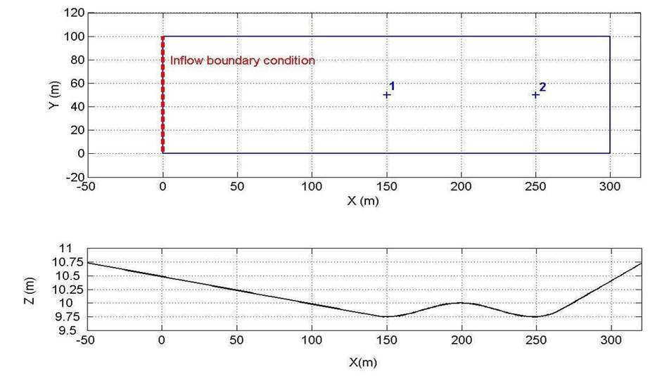
Figure 3.1. A) Plan view of channel with boundary condition and sampling points annotated; B) Profile view of channel showing slopes and internal obstruction.
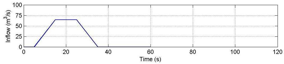
Figure 3.2. Inflow hydrograph applied at the left-hand side of the 2D area.
Points 1 and 2 are located at X = 150m and X = 250m, respectively. The simulation time step was 1s and the reporting resolution was every 5s for the 15min simulation duration. Water levels and velocities were both reported for this test case that emphasized momentum conservation.
The DEM (from the UK EA reference documents) was imported into a new AquaTwin project. The 2D boundary was initialized as a 300m x 100m rectangular polygon. The default roughness was specified to be 0.01 and there was no infiltration. Meshing options were calibrated to achieve grid resolution (~1200 nodes) recommended by the test.
A guideline polygon layer was added such that the intersection corresponded with Points 1 and 2. The boundary condition was applied as an inflow boundary on the left-hand side of the channel. The simulation was run at a 1s time step.
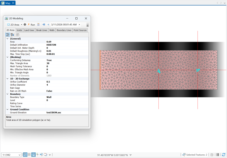
Figure 3.3. AquaTwin modeling parameters and interface. Selected mesh elements correspond with sampling points 1 and 2.

Figure 3.4. AquaTwin Sewer 2D – Flood Viewer 3D rendering of flood wave condition at T=265s. Dark blue indicates deeper water. DEM is exaggerated 5.0x to sharpen vertical relief.
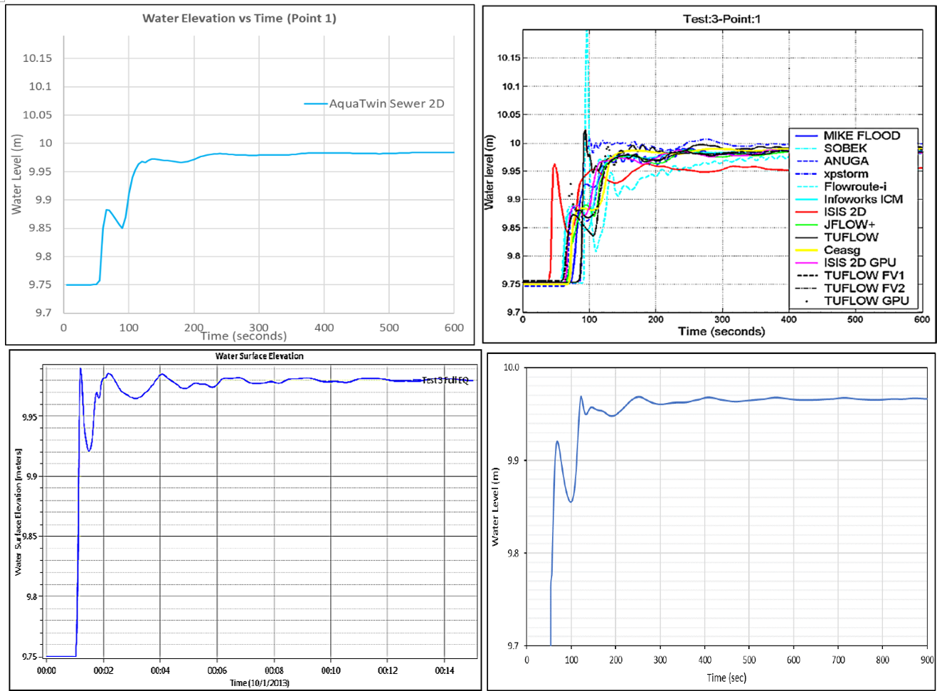
Figure 3.5. Point 1 WSE. Top left: AquaTwin. Top right: Ensemble, reproduced from Néelz and Pender (2013); as it appears in Kramer (2021), p. 4-5. Bottom left: HEC-RAS, reproduced from Brunner (2018); as it appears in Kramer (2021), p. 4-5. Bottom right: SRH-2D, reproduced from Kramer (2021), p. 4-5.
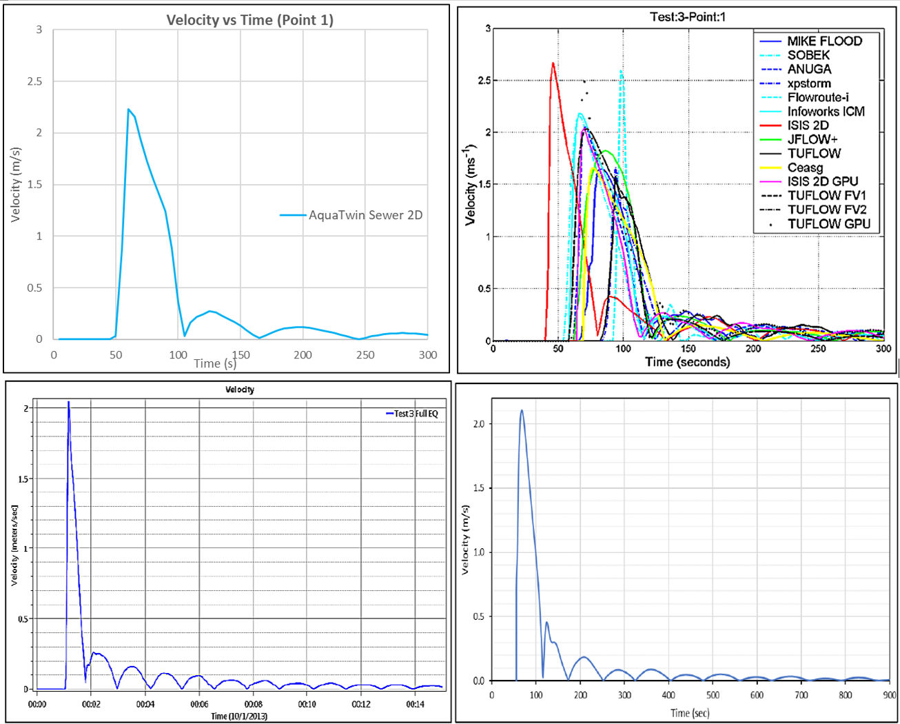
Figure 3.6. Point 1 Velocity. Top left: AquaTwin. Top right: Ensemble, reproduced from Néelz and Pender (2013); as it appears in Kramer (2021), p. 4-6. Bottom left: HEC-RAS, reproduced from Brunner (2018); as it appears in Kramer (2021), p. 4-6. Bottom right: SRH-2D, reproduced from Kramer (2021), p. 4-6.
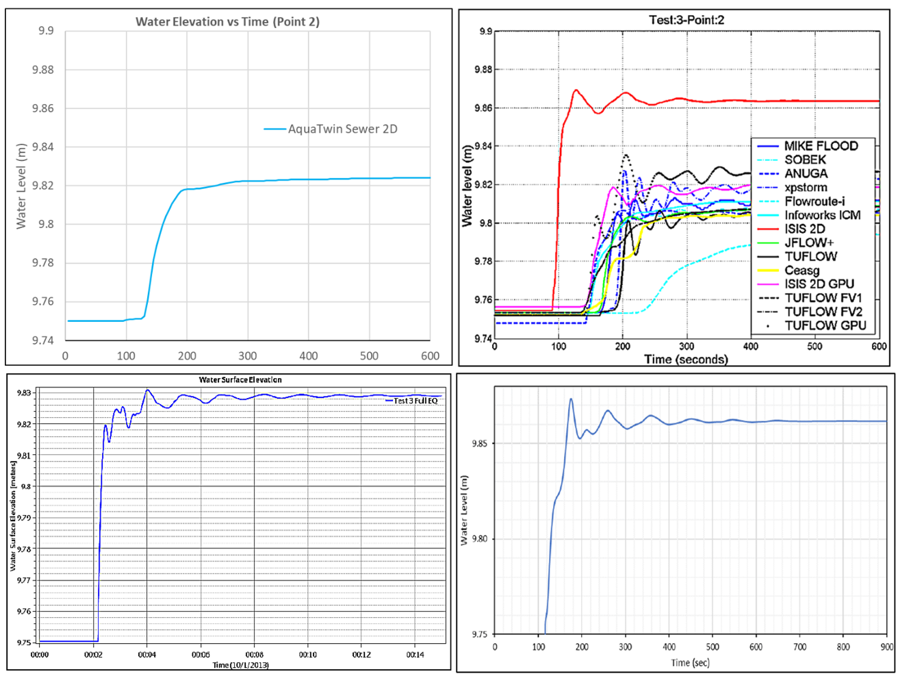
Figure 3.7. Point 2 WSE. Top left: AquaTwin. Top right: Ensemble, reproduced from Néelz and Pender (2013); as it appears in Kramer (2021), p. 4-5. Bottom left: HEC-RAS, reproduced from Brunner (2018); as it appears in Kramer (2021), p. 4-5. Bottom right: SRH-2D, reproduced from Kramer (2021), p. 4-5.
Note: Velocities at Point 2 were not provided by Néelz and Pender (2013) and were similarly omitted from this report.
WSE: At Point 1, ahead of the obstruction, AquaTwin, HEC-RAS (Full EQ), SRH-2D, and several models in the Ensemble (including TUFLOW, ICM, and MIKE FLOOD) all show the same transient: a rapid rise as the flood pulse arrives, a period of post-arrival oscillation, and a settling to a quasi-steady plateau around 9.97–9.98.
Point 2 exists at the elevation nadir on the far side of the obstruction. AquaTwin’s rise is relatively smooth, aligning with TUFLOW, ICM, and MIKE FLOOD in the Ensemble. HEC-RAS, SRH-2D, and other Ensemble models (including ISIS 2D, ANUGA, and XPSTORM) all carry more pronounced oscillations. More notable than the shape difference is where each solver ends up. AquaTwin and HEC-RAS converge to nearly the same final level at Point 2 (~9.82 m and ~9.83 m, respectively), while SRH-2D stabilizes roughly 0.03 m higher. This isn’t just an AquaTwin/HEC-RAS-vs-SRH-2D split: within the Ensemble, most packages (TUFLOW, MIKE FLOOD, ANUGA, and others) also settle in the 9.80–9.82 m range alongside AquaTwin, while ISIS 2D is the clear outlier at ~9.86 m, tracking with SRH-2D’s higher plateau instead.
Because Point 2 sits just past the internal obstruction, its final level is effectively a record of how much flow volume made it over the hill rather than remaining upstream at Point 1. A lower final level at Point 2 implies less overtopping volume — consistent with a numerical scheme that dissipates more of the flood pulse’s momentum before it crests the obstruction.
Velocity: The flood wave is predicted by AquaTwin to arrive at Point 1 around the 50s mark, with velocity peaking around ~2.2 m/s a few seconds later. This velocity timing and magnitude match neatly with HEC-RAS, SRH-2D, and full-SWE models in the Ensemble, especially ICM. ISIS 2D GPU and TUFLOW arrive one or two seconds later. The oscillation that was observed in the WSE at Point 1 was also seen in the velocity, where a ~50s period wave was seen that dampened quickly (never again reaching 0.5 m/s). SRH-2D and HEC-RAS retained the most reflected velocity; AquaTwin’s velocity profile was nestled between those solvers and several Ensemble models, nearly matching those from ICM, ISIS 2D GPU, and TUFLOW.
Velocity results for Point 2 were not provided by any of the reference reports and, for consistency, were also not included in this comparison.
Test Case 4 evaluates a modeling package’s ability to simulate the celerity of a flood wave propagating across an open, frictional terrain. The domain (Figure 4.1) is a flat, horizontal floodplain measuring 1000 m x 2000 m at a uniform ground level of 0 m. An inflow boundary condition is applied along a 20 m segment at the midpoint of the western edge, representing the failure of a flood defense by breaching or overtopping. The inflow hydrograph peaks at 20 m3/s with a base time of approximately 5 hours. All other domain boundaries are walls (no flow across), and the floodplain starts completely dry.
A uniform Manning’s roughness of n = 0.05 is applied across the domain. The prescribed resolution is ~80,000 computational elements across the modeled area, and the simulation is set to run for 5 hours.
This test isolates wave celerity and depth/velocities at the leading edge of the advancing flood front from any complicating topographic effects. The simulation time and domain extent are such that the leading edge is not expected to interact with the domain’s wall boundaries.
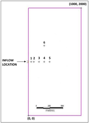
Figure 4.1. 2D domain for Test Case 4 along with Inflow Location and Sample Point locations. The DEM is uniform at 0 m.

Figure 4.2. Screenshot of inflow boundary condition constructed in AquaTwin.
Points 1 – 5 fall on a line orthogonal to the center of the boundary condition to assess the depth and velocity of the advancing flood wave; Point 6 is aligned with Point 4 and is intended to capture the spread of the flood wave across the uniformly flat 2D floodplain.
For concision, WSE and velocities for Points 3 and 6 only are included herein. Additionally, a WSE profile at t = 1hr is presented. To review the comparison against all reference points, please see Appendix A.4.
The DEM (from the UK EA reference documents) was imported into a new AquaTwin project (though the DEM is uniform at 0 m, AquaTwin still requires a DEM raster to generate the mesh). The 2D boundary was initialized as a 1000 m x 2000 m rectangular polygon with wall boundaries. The default roughness was 0.05 and there was no infiltration. Meshing options were calibrated to achieve the recommended grid resolution (~80,000 elements).
A guideline polygon layer was added such that the intersections corresponded with Points 1 – 6. The boundary condition was applied as an inflow boundary along a 20 m segment on the western edge of the domain. The simulation was run at a 1s time step.

Figure 4.3. Screenshot of the Test Case 4 setup in AquaTwin. The grey domain reflects the high-resolution of computational elements; the cyan triangles are selected elements that represent the sample points. The inflow boundary condition is shown in orange.
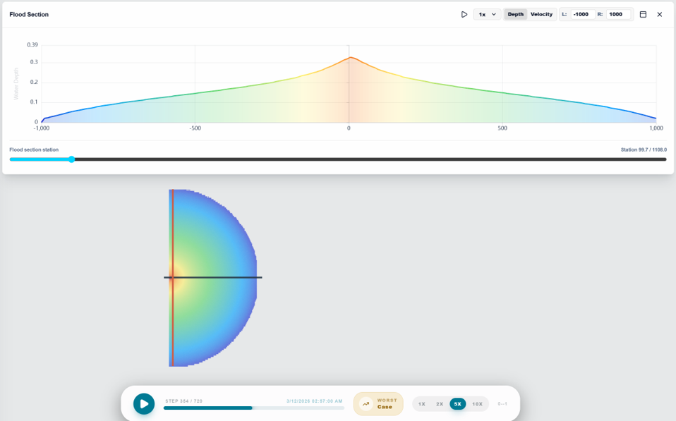
Figure 4.4. AquaTwin Sewer 2D – Flood Viewer plan view and section view of flood wave depth at t = ~3 hrs. A) Flood section at station = ~100 m from input boundary extending 1000 m in each direction from the input boundary centerline; B) Plan view of semicircular propagation of floodwave across the plain, red indicates greater depth while blue indicates the water’s leading edge.
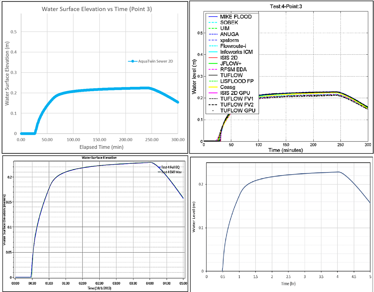
Figure 4.5. Point 3 WSE. Top left: AquaTwin. Top right: Ensemble, reproduced from Néelz and Pender (2013); as it appears in Kramer (2021), p. 5-10. Bottom left: HEC-RAS, reproduced from Brunner (2018); as it appears in Kramer (2021), p. 5-10. Bottom right: SRH-2D, reproduced from Kramer (2021), p. 5-10.

Figure 4.6. Point 3 Water Velocity. Top left: AquaTwin. Top right: Ensemble, reproduced from Néelz and Pender (2013); as it appears in Kramer (2021), p. 5-11. Bottom left: HEC-RAS, reproduced from Brunner (2018); as it appears in Kramer (2021), p. 5-11. Bottom right: SRH-2D, reproduced from Kramer (2021), p. 5-11.
Figure 4.7. Point 6 WSE. Top left: AquaTwin. Top right: Ensemble, reproduced from Néelz and Pender (2013); as it appears in Kramer (2021), p. 5-16. Bottom left: HEC-RAS, reproduced from Brunner (2018); as it appears in Kramer (2021), p. 5-16. Bottom right: SRH-2D, reproduced from Kramer (2021), p. 5-16.

Figure 4.8. Point 6 Water Velocity. Top left: AquaTwin. Top right: Ensemble, reproduced from Néelz and Pender (2013); as it appears in Kramer (2021), p. 5-17. Bottom left: HEC-RAS, reproduced from Brunner (2018); as it appears in Kramer (2021), p. 5-17. Bottom right: SRH-2D, reproduced from Kramer (2021), p. 5-17.
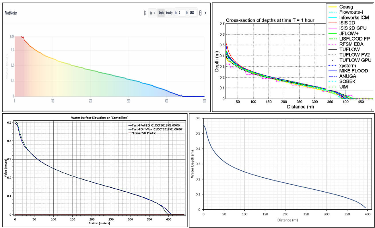
Figure 4.9. Cross Section from Inflow to Point 5, WSE vs Distance at T=1hr. Top left: AquaTwin. Top right: Ensemble, reproduced from Néelz and Pender (2013); as it appears in Kramer (2021), p. 5-18. Bottom left: HEC-RAS, reproduced from Brunner (2018); as it appears in Kramer (2021), p. 5-18. Bottom right: SRH-2D, reproduced from Kramer (2021), p. 5-18.
WSE: At Point 3, AquaTwin’s rise begins around t = ~30 min and reaches a broad, mildly increasing plateau around 0.2 m that increases to ~0.23 m before declining around t = 240 min. This shape and timing are largely preserved by HEC-RAS, SRH-2D, and all models in the Ensemble. By Point 6, farther from the inflow, the arrival is delayed to around t = ~70 min, and the peak is slightly attenuated, but the same rough shape is observed. The WSE from AquaTwin’s peaks around ~0.17 m, which is consistent with HEC-RAS, SRH-2D, and all models in the Ensemble.
Figure 4.9 shows the WSE profile (rather than time series) from the inflow location to Point 5 at t = 1 hr. AquaTwin’s profile shape agrees well with the S-curves shown in the reference plots, starting around ~0.5 m and the edge of the wave around 400 m.
Velocity: In slight contrast to the WSE, the velocity of the flood wave leading edge arrives more suddenly. The velocity wave arrives at Point 3 around t = ~30 s and peaks around ~0.16 m/s for AquaTwin, HEC-RAS, SRH-2D, and several key Ensemble models such as TUFLOW and ICM (though the spread of the Ensemble models is larger for velocity than for water depth). Similarly, the wave’s velocity arrives at Point 6 in a sharp ascent to ~0.1 m/s just after the t = 1 hr mark, with close agreement between AquaTwin, HEC-RAS, SRH-2D, and the full-SWE models in the Ensemble.
Notably, HEC-RAS’s Full EQ and Diffusive Wave solutions are essentially indistinguishable in Test Case 4, which contrasts with their moderate water level disagreement in Test Case 2.
Test Case 5 evaluates a modeling package’s ability to simulate major flood inundation and predict flood hazard following a dam failure. Specifically, peak water levels, velocities, and travel times of a flood wave in a large, natural river valley (Figure 5.1). The modeled domain is a real-world river valley in Scotland, UK measuring approximately 0.8 km wide and 17 km long, sloping downstream at roughly 1:100 in its upper reach and easing to roughly 1:1000 in the lower reach.
A single inflow boundary condition is applied along a ~260 m line at the upstream end of the valley, representing the failure of a dam structure. The inflow hydrograph (Figure 5.2) is a skewed trapezoidal shape with a short, sharp early peak of 3,000 m3/s. All other domain boundaries are walls (no-flow) and the domain starts completely dry. A uniform Manning’s roughness of n = 0.04 is applied across the domain. The nominal grid resolution is ~50 m (~7,600 nodes across the ~19 km2 modeled area).
The domain scale and slope gradient (including channel cross-sectional topographic complexity) in Test Case 5 is well beyond anything tested in Test Cases 1 – 4. Additionally, the inflow magnitude is several orders of magnitude higher than anything yet tested. This test case is designed to produce both supercritical and subcritical flow regimes within the same domain, an important benchmark for any SWE solver.

Figure 5.1. 2D domain boundary superimposed on grey-scale DEM of natural river valley. Sample point locations, inflow boundary condition, and channel centerline annotated.
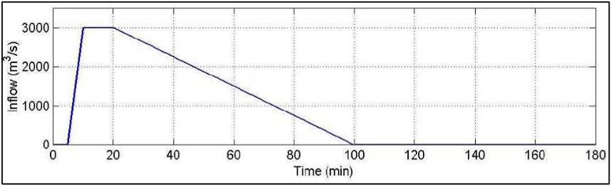
Figure 5.2. Inflow boundary condition timeseries representing a simulated dam-break flood wave.
Seven output points are distributed along the valley at increasing distance downstream from the dam; Points 1 – 5 are on the channel centerline, while Points 6 & 7 are horizontally offset from the centerline (Figure 5.1). WSE and velocity are reported at each point at an output interval of 60 s for a 30 hr simulation duration (long enough for the water to settle in the lower reach of the valley).
For concision, only WSE and velocity for Point 1 & Point 7 are included herein. See Appendix A.5 for the full suite of sample point output figures.
The DEM (from the UK EA reference documents) was imported into a new AquaTwin project. Unlike the DEMs from Test Case 1 – 4, Test Case 5 is a real location, a river valley in the highland lochs region of Scotland; the British National Grid coordinate system was used (EPSG: 27700). The UK EA reference documents also included shapefiles for the 2D domain boundary, boundary condition location, and the sampling point locations. The default roughness was 0.04 and there was no infiltration permitted throughout the domain. Meshing options were calibrated to achieve the recommended grid resolution (~7600 elements). The simulation was run at a 2s time step.
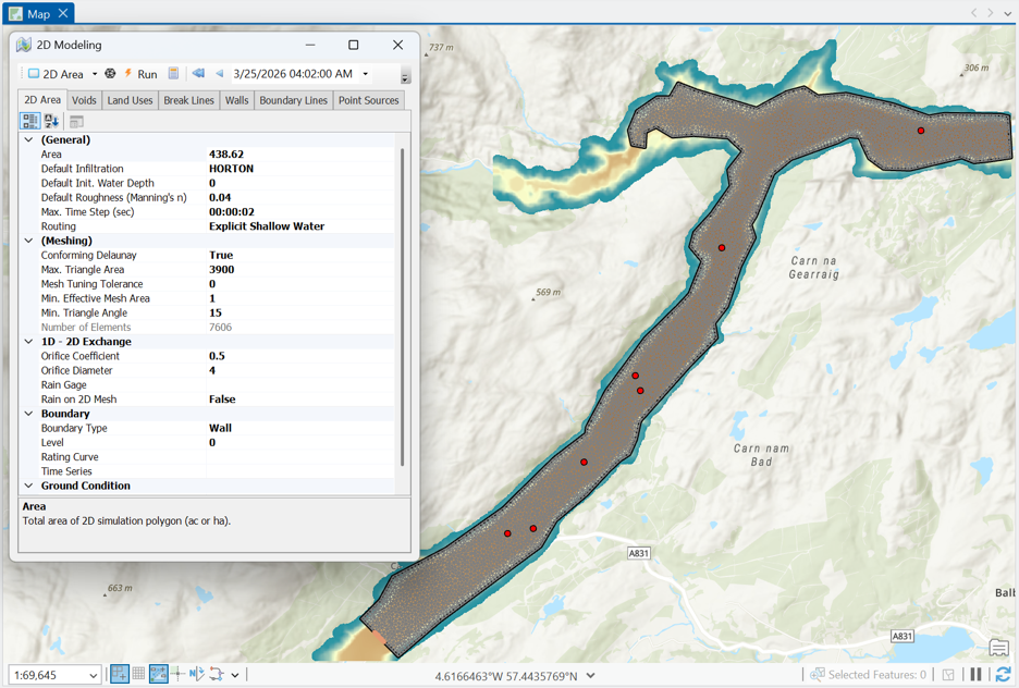
Figure 5.3. Screenshot of Test Case 5 modeling domain constructed in AquaTwin; the simulation mesh, domain boundary (black), inflow boundary condition location (orange), and sampling point locations (red) are superimposed on the DEM. The satellite imagery basemap shows this real-world river valley near Carn nam Bad Mountain in Scotland, UK.

Figure 5.4. AquaTwin Sewer 2D – Flood Viewer 3D rendering of the simulated domain with hillshading to highlight vertical relief. “Worst Case” flood inundation shows maximum water depths during the simulation.

Figure 5.5. Point 1 WSE. Top left: AquaTwin. Top right: Ensemble, reproduced from Néelz and Pender (2013); as it appears in Kramer (2021), p. 6-5. Bottom left: HEC-RAS, reproduced from Brunner (2018); as it appears in Kramer (2021), p. 6-5. Bottom right: SRH-2D, reproduced from Kramer (2021), p. 6-5.
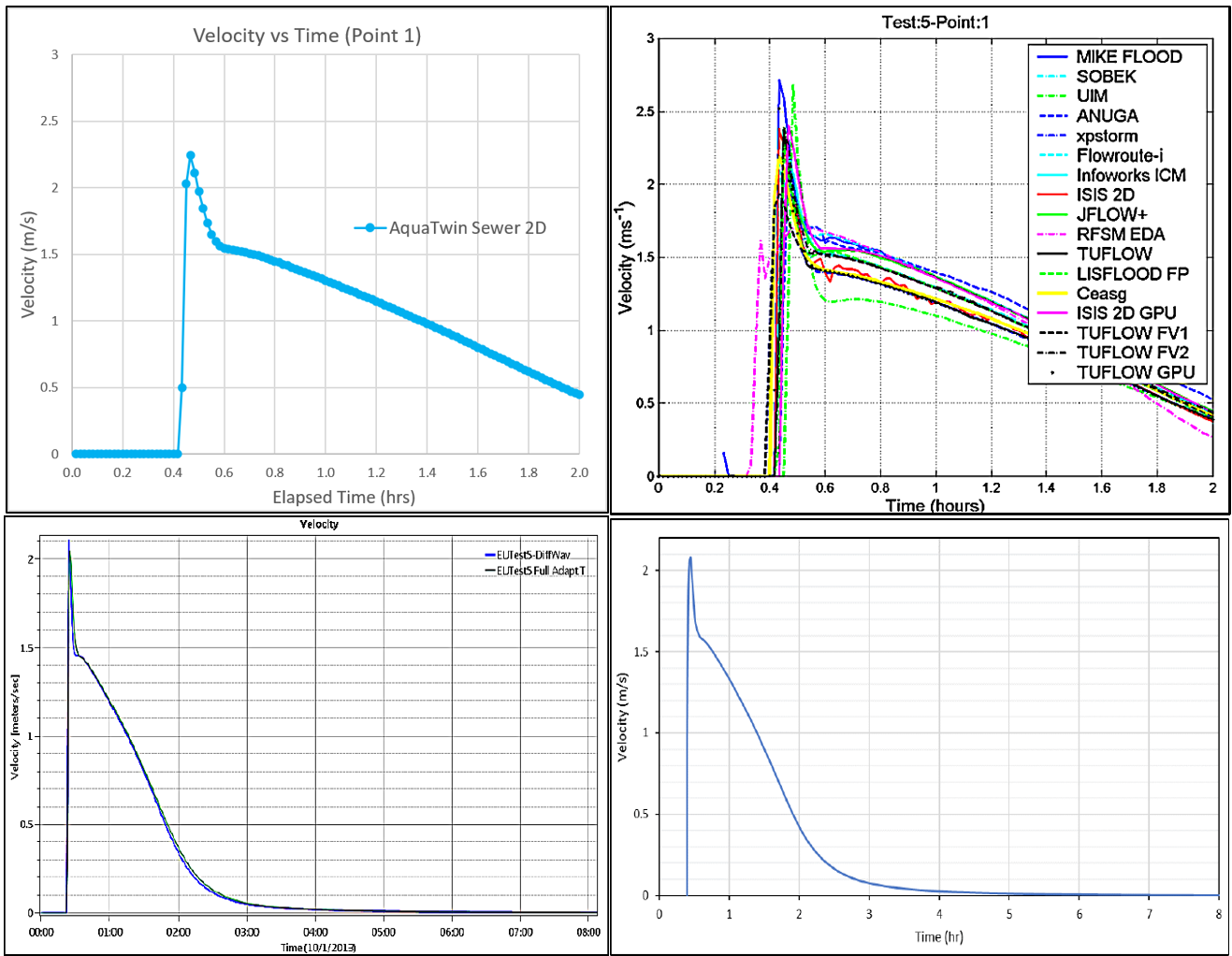
Figure 5.6. Point 1 Water Velocity. Top left: AquaTwin. Top right: Ensemble, reproduced from Néelz and Pender (2013); as it appears in Kramer (2021), p. 6-6. Bottom left: HEC-RAS, reproduced from Brunner (2018); as it appears in Kramer (2021), p. 6-6. Bottom right: SRH-2D, reproduced from Kramer (2021), p. 6-6.
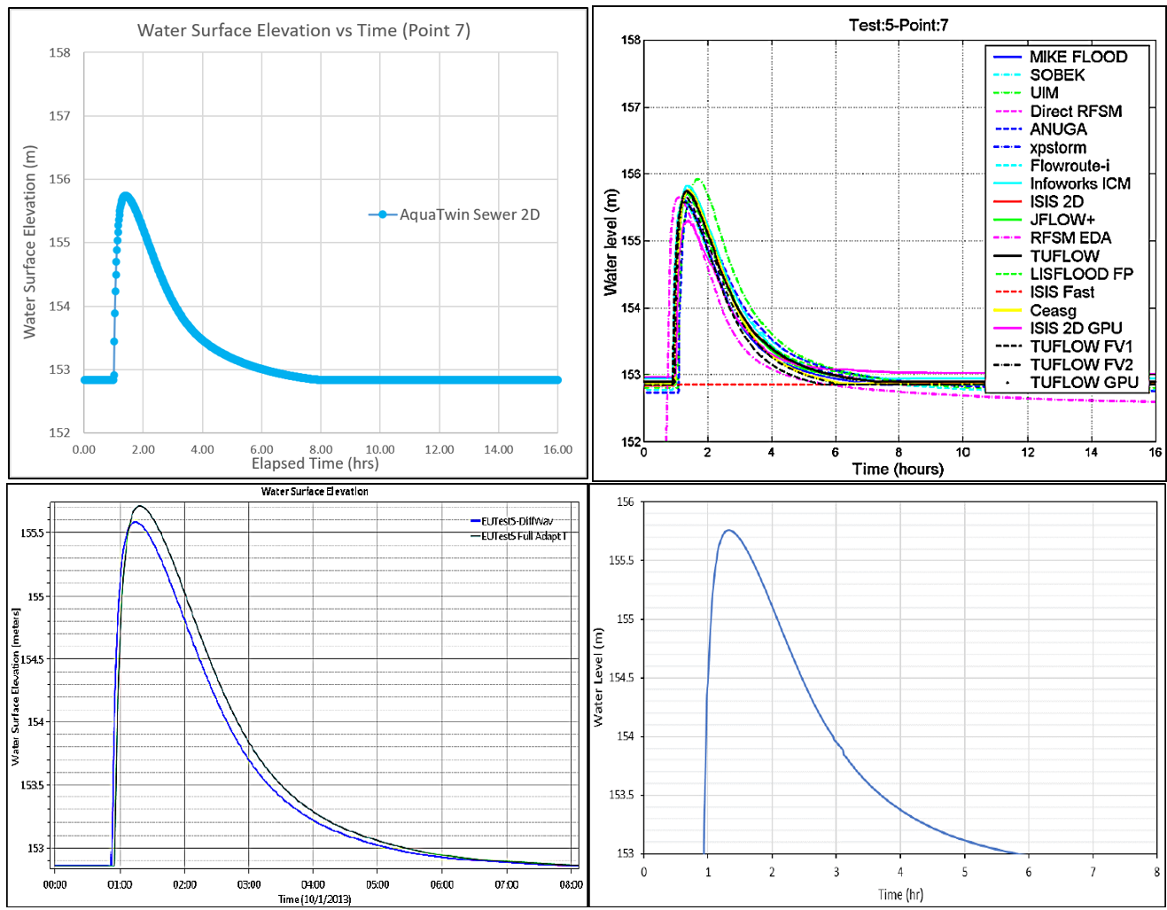
Figure 5.7. Point 7 WSE. Top left: AquaTwin. Top right: Ensemble, reproduced from Néelz and Pender (2013); as it appears in Kramer (2021), p. 6-17. Bottom left: HEC-RAS, reproduced from Brunner (2018); as it appears in Kramer (2021), p. 6-17. Bottom right: SRH-2D, reproduced from Kramer (2021), p. 6-17.

Figure 5.8. Point 7 Water Velocity. Top left: AquaTwin. Top right: Ensemble, reproduced from Néelz and Pender (2013); as it appears in Kramer (2021), p. 6-18. Bottom left: HEC-RAS, reproduced from Brunner (2018); as it appears in Kramer (2021), p. 6-18. Bottom right: SRH-2D, reproduced from Kramer (2021), p. 6-18.
WSE: At Point 1, near the inflow boundary condition, AquaTwin’s wave arrives at t = ~0.4 hr and peaks around ~174.8 m at the t = ~0.6 hr mark. Following the peak, the receding limb stabilizes around ~172.3 m by t = ~4 hr. This wave arrival timing, peak magnitude, and receding limb shape track very closely with SRH-2D and HEC-RAS FEQ, MIKE FLOOD, TUFLOW, ISIS 2D, and JFLOW+. The full Ensemble has some spread about the peak magnitude, but the full-SWE models listed above tend to agree. All four panels converge to the same ~172.3 m plateau as AquaTwin.
At Point 7, further downstream and slightly off the channel centerline, at Point 7, AquaTwin’s wave arrives at almost exactly the t = 1 hr mark, quickly peaking at ~155.8 m. Similar to Point 1, the flood wave timing and peak are nearly coincident with the other full-SWE models, including SRH-2D (~155.75 m), HEC-RAS FEQ (~155.7 m), and the main Ensemble cluser (MIKE FLOOD, TUFLOW, ISIS 2D, JFLOW+). Unlike Point 1, there is no residual water retained up the channel side slope at Point 7, nearly all models in Figure 5.13 show a return to the ~152.9 m baseline by t = ~8 hrs.
Velocity: The arrivals of the flood wave in the Velocity time series are marked by a very sudden increase from the 0 m/s baseline to the peak. At Point 1, AquaTwin predicted the peak at ~ 2.25 m/s just after t = 0.4 hr. The velocity quickly drops to ~1.5 m/s before approximately linearly decreasing over the next 1.5 hrs. The shape of AquaTwin’s velocity curve is precisely echoed by all reference models, with tight agreement on both the timing and peak velocity by SRH-2D, HEC-RAS, and several of the Ensemble models, including TUFLOW, ISIS 2D, and ICM (MIKE FLOOD is an outlier here, predicting > ~2.5 m/s peak velocity). The full-SWE models vary by ~0.2 m/s on the receding limb velocity; AquaTwin’s prediction is about the average of all comparison models.
By Point 7, the leading edge of the flood wave has attenuated slightly. The timing of the arrival (t = ~1 hr) is agreed upon by nearly all models, though there is variability among the predicted peak magnitude at this point. AquaTwin’s predicted peak velocity of ~1.38 m/s matches the predictions from SRH-2D, HEC-RAS FEQ, and a cluster of Ensemble models including TUFLOW, JFLOW+, and ICM. ISIS 2D GPU is an outlier here, showing some instability around a peak near 2.0 m/s.
Notably, several of the diffusion wave solvers, including HEC-RAS Diff Wave and LISFLOOD, predicted higher peak velocities at Point 7 than their full-SWE counterparts.
Across both points and both metrics, AquaTwin‘s arrival timing, peak timing/magnitude, and recession shape land consistently within the HEC-RAS/SRH-2D/core-Ensemble envelope — the expected result for a test dominated by momentum-conserving wave propagation down a sloped valley, which is squarely the regime full-SWE solvers are built to handle consistently.
Unlike Test Cases 1 – 5, which compare AquaTwin simulation predictions against other numerical models only, Test Case 6A also includes physical measurements. Test Case 6A is the original dam-break test case developed for the IMPACT project (Soares-Frazão and Zech, 2002), based on a physical flume model built at the Civil Engineering Laboratory of the Université Catholique de Louvain (UCL). All dimensions in this benchmark reflect the laboratory scale of that physical model (Figure 6.1).
A 3.60 m wide flume with a 6.75 m long reservoir is initialized to a depth of 0.4 m. This reservoir is separated from a downstream channel by a dam wall containing a 1 m wide gate opening centered in the flume. The downstream channel is initialized at a uniform depth of 0.02 m and extends 99 m downstream of the gate (such that the downstream boundary condition does not factor into the simulation). A rectangular block obstruction is placed 3.44 m downstream of the gate, slightly off center. The block, measuring 0.8 m x 0.4 m, is at a 64º angle with the gate. At t = 0, the gate is instantaneously removed, releasing the reservoir into the downstream channel and producing a rapidly advancing wave that impinges asymmetrically on the block. The flume is completely flat; flow is driven by the initial head difference between the two sides of the gate.
A uniform Manning’s roughness of n = 0.01 is applied throughout, consistent with the smooth surface typical of a laboratory flume. The nominal grid resolution is 0.1 m (~36,000 computational elements), by far the finest resolution used in any Test Case in this benchmarking suite. The simulation is run to t = 2 min, though the comparison of primary interest is the first 60 s of simulation time.
The objective of this test case is to assess a modeling package’s ability to simulate hydraulic jumps and wake zones that occur when the flood wave interacts with the block. This high-resolution case is a substantially more demanding test of shock-capturing than Test Case 3’s momentum conservation obstruction, both because of the instantaneous release of the reservoir (as opposed to a gradual hydrograph) and because measurement data exist against which to ground the numerical model results.
A key reference model, HEC-RAS (FEQ) was not provided for this super high-resolution Test Case 6A, but is included in the scaled-up version (Test Case 6B).
Six gauge points (G1 – G6) are positioned around the gate and block (Figure 6.1): G6 sits in the reservoir upstream of the gate; G1 and G2 sit just downstream of the gate on either side of the flume centerline; G3 and G4 sit farther downstream, flanking the building; and G5 sits immediately behind the building, in the wake zone. WSE and velocity timeseries are reported for each location at a 1s time resolution, the highest resolution possible with AquaTwin.
Additionally, maximum WSE was reported along two cross-sections that capture the shape of the hydraulic jump and wake zones (Figure 6.2).
For concision, the time series comparison figures for only Points G2, G4, G6, as well as the cross-sectional profiles, were included herein. See Appendix A.6 for the full suite of comparison figures.

Figure 6A.1. Detailed schematic of the Test Case 6 experimental flume from Soares-Frazão and Zech (2002).

Figure 6A.2. Plan view of the flume illustrating relative locations for cross-sections XS1 and XS2.
The flume DEM (from the UK EA reference documents) was imported into a new AquaTwin project. Measurements from Figure 6.1 were used to define a point feature class for the sample point locations, as well as the gate and obstructing block. Two land use refinement zones were used to create the variable initial conditions on either side of the gate. Dam walls and obstructing block were represented as voids, excluding their area from the meshing. The roughness was 0.01 for the whole domain, and no infiltration was permitted. Meshing options were consistent between the refinement zones and were calibrated to achieve the recommended grid resolution (~36,000 computational elements). The simulation was run at a 0.1s time step, though the minimum possible reporting time was 1s.
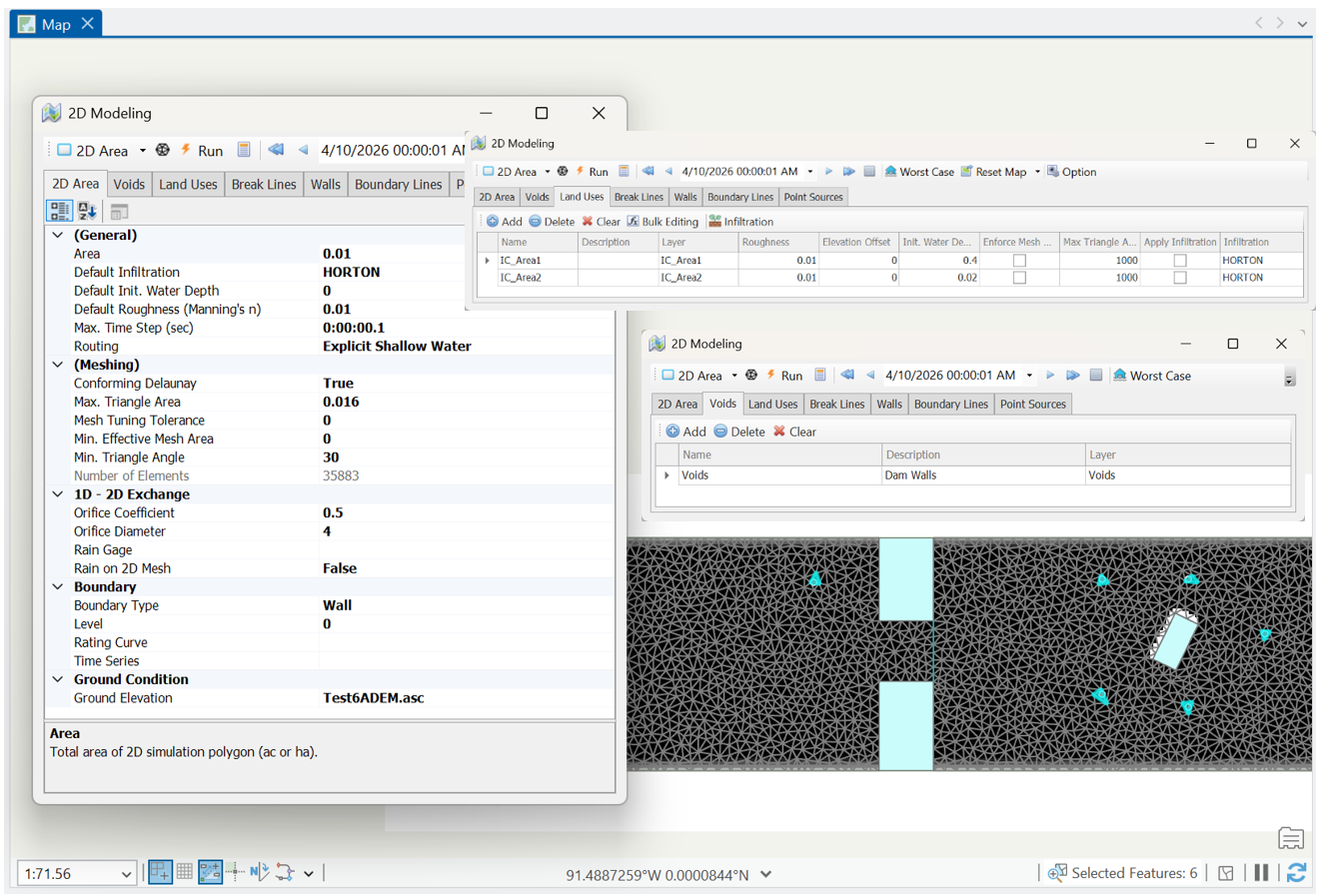
Figure 6A.3. Screenshot of Test Case 6 constructed in the AquaTwin interface. Triangular mesh elements corresponding to sampling points are selected. Simulation parameters, refinement zone areas, and void layers are shown.

Figure 6A.4. Water depths from AquaTwin during the first few seconds of the simulation, A) t = 0s; B) t = 1s; C) t = 10s. Deepest blue is 0.4 m, lightest blue is 0.02 m; dam and blocks in red, weir gate in green, Points G1 – G6 in pink.

Figure 6A.5. Point G2 WSE. Top left: AquaTwin. Top right: Ensemble, reproduced from Néelz and Pender (2013); as it appears in Kramer (2021), p. 7-6. Bottom left: SRH-2D, reproduced from Kramer (2021), p. 7-6.

Figure 6A.6. Point G2 Velocity. Top left: AquaTwin. Top right: Ensemble, reproduced from Néelz and Pender (2013); as it appears in Kramer (2021), p. 7-7. Bottom left: SRH-2D, reproduced from Kramer (2021), p. 7-7.

Figure 6A.7. Point G4 WSE. Top Left: AquaTwin Sewer 2D. Top right: Ensemble, reproduced from Néelz and Pender (2013); as it appears in Kramer (2021), p. 7-9. Bottom Left: SRH-2D, reproduced from Kramer (2021), p. 7-9.

Figure 6A.8. Point G4 Velocity. Top Left: AquaTwin Sewer 2D. Top right: Ensemble, reproduced from Néelz and Pender (2013); as it appears in Kramer (2021), p. 7-10. Bottom Left: SRH-2D, reproduced from Kramer (2021), p. 7-10.
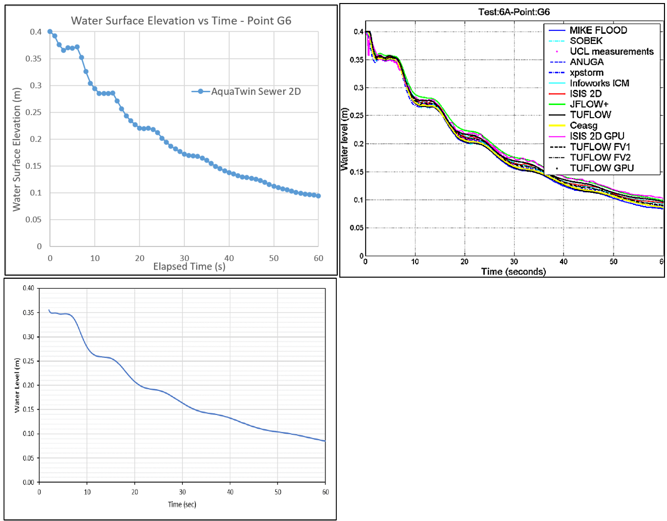
Figure 6A.9. Point G6 WSE. Top left: AquaTwin. Top right: Ensemble, reproduced from Néelz and Pender (2013); as it appears in Kramer (2021), p. 7-13. Bottom left: SRH-2D, reproduced from Kramer (2021), p. 7-13.
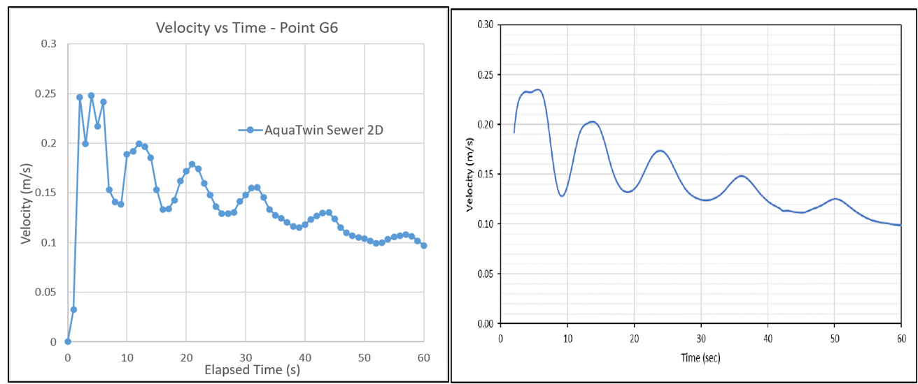
Figure 6A.10. Point G6 Velocity. Left: AquaTwin. Right: SRH-2D, reproduced from Kramer (2021), p. 7-14.

Figure 6A.11. Profile XS1 Maximum Water Level. Left: AquaTwin. Right: SRH-2D, reproduced from Kramer (2021), p. 7-16.
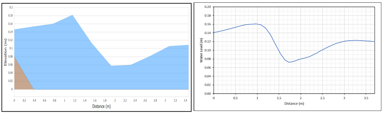
Figure 6A.12. Profile XS2 Maximum Water Level. Left: AquaTwin. Right: SRH-2D, reproduced from Kramer (2021), p. 7-17.
Reservoir gauge (G6): The WSE at G6, upstream of the flume gate, shows a periodic recession (Figure 6A.9). This staircase decline is reproduced almost exactly by AquaTwin, SRH-2D, and the tight Ensemble cluster including the direct measurements from the UCL experiment.
Velocity at G6 shows a similar strong agreement with SRH-2D (velocity was not reported by the Ensemble or recorded in the UCL experiment). AquaTwin’s version of the velocity curve has a slightly higher frequency in the decaying oscillation, but the underlying pattern is the same (Figure 6A.10).
Wake-zone gauge (G4): The wake-zone immediately downstream of the obstructing block is a key location for this test case. The timing of the wake development as well as the peak WSE are perhaps the most important outcomes from this benchmark test case. The WSE from AquaTwin is predicted to spike quickly to ~0.12 m by t = 4-5 s and fully develop at ~0.13 m by the 10 s mark. This water peak magnitude and timing matches neatly with SRH-2D and the Ensemble, including the UCL measurements. All models show a slightly wavy recession as the reservoir empties, agreeing that the water level has reduced to ~0.6 m by t = 60 s. The Ensemble models show some variability on the exact water level during the recession limb, though AquaTwin can be seen to track closely with TUFLOW and ICM (among others) after about the 20 s mark (Figure 6A.7).
Near-gate gauge (G2): The WSE and velocity time series results for the sample points downstream of the reservoir gate shows the most variability of any benchmark case so far. At point G2, there is an almost immediate water level surface spike (1-2s at ~0.1 m) predicted by several of the models, including AquaTwin, SRH-2D, TUFLOW, ISIS 2D, and, importantly, reflected in the observations from the UCL experiment. Other models like ICM and MIKE FLOOD show the spike happening seconds later or not at all. The WSE’s ultimate peak around ~0.14 m is predicted to occur by the 10 s mark by AquaTwin, which matches most nearly with the expectations of JFLOW+, TUFLOW, and ISIS 2D. Other models, including SRH-2D and TUFLOW GPU, lag behind AquaTwin, though nearly every model is early compared to the measured results from the UCL experiment. The exceptions are Ceasg, SOBEK, and TUFLOW FV1 and FV2, which have been outliers on other test cases (Figure 6A.5).
The velocity timeseries shape shows a pattern of an initially high velocity pulse as the initial gate wave passes through, followed by an equally sharp decline, and then bumpy rise and fall as the standing hydraulic jump stabilizes. AquaTwin’s initial wave velocity matches that predicted by SRH-2D and most of the Ensemble models, as well as the data from the UCL experiment (Figure 6A.6). After the initial wave, there is much less agreement between any of the models; most show a similar qualitative shape to AquaTwin, but there is a wide spread of timings and magnitudes. Importantly, the UCL experiment data shows nearly as much noise as the Ensemble models, so it is hard to draw meaningful conclusions about the velocity at Point G2 after about the 12s mark. Specific differences between each modeling package with regards to the 2D area discretization scheme may be dominating the results.
Cross-Sections: The cross-sectional profiles of maximum WSE were compared between AquaTwin and SRH-2D, as they were not provided by the Néelz and Pender (2013) report. Both models exhibit similar patterns: wave peak and trough magnitudes are within ~0.2m and locations are within half a meter (Figs 6A.11 and 6A.12). The cross-sections were not precisely specified in the test description, so slight differences in the profile paths between AquaTwin and SRH-2D likely dominate differences (especially spatial differences) in the results.
Some other conditions may impact the results of this complicated, high-resolution scenario. AquaTwin’s triangular mesh reports a cell-averaged value for the mesh element that corresponds with the precise sample location, which can create a slight offset to the location of the hydraulic jump and wake zone. Additionally, AquaTwin specifies the initial condition as a water depth, rather than an elevation. This creates a slight elevation gradient near the sloped flume edges (see Figure 6A.1), which contributes cross-sectional wave behavior in the simulation that does not exist in the real-world flume.
Test Case 6B uses the identical geometry, gate configuration, and obstruction layout as Test Case 6A (Figure 6A.1), with every physical dimension scaled up by a factor of 20 – converting the laboratory flume into a “field-scale” domain intended to reflect dimensions more typical of practical flood inundation modeling.
Initial conditions scale accordingly: a uniform depth of 8 m upstream of the dam and 0.4 m downstream (versus 0.4 m and 0.02 m in Test Case 6A). A uniform Manning’s roughness of n = 0.05 is applied throughout, reflecting a more realistic field surface rather than a smooth laboratory flume. The nominal grid resolution is 2 m (~36,000 nodes, the same node count as 6A at 20× the resolution), and the simulation is run to t = 30 min, compared to t = 2 min for Test Case 6A.
Gauge locations (G1–G6) and reported quantities are unchanged in principle from Test Case 6A, scaled to the new geometry; output frequency is 1 s, versus 0.1 s in Test Case 6A. Cross-sectional profiles for WSE are drawn in the corresponding locations to Test Case 6A.
Data for Points G2 and G4 only are included in the main body of this report. For the full set of results at all gauge locations, see Appendix section A7.
The scaled-up DEM (from the UK EA reference documents) was imported into a new AquaTwin project. Measurements from Figure 6.1 were magnified by 20x and used to define a point feature class for the sample point locations, as well as the gate and obstructing block. Two land use refinement zones were used to create the variable initial conditions on either side of the gate. Dam walls and obstructing block were represented as voids, excluding their area from the meshing. The roughness was 0.05 for the whole domain, and no infiltration was permitted. Meshing options were consistent between the refinement zones and were calibrated to achieve the recommended grid resolution (~36,000 computational elements). The simulation was run at a 0.25s time step; the reporting time was 1s.

Figure 6B.1) Point G2 WSE. Top Left: AquaTwin Sewer 2D. Top Right: Ensemble, reproduced from Néelz and Pender (2013); as it appears in Kramer (2021), p. 7-23. Bottom Left: HEC-RAC FEQ, reproduced from Brunner (2018); as it appears in Kramer (2021), p. 7-23. Bottom Right: SRH-2D, reproduced from Kramer (2021), p. 7-23.
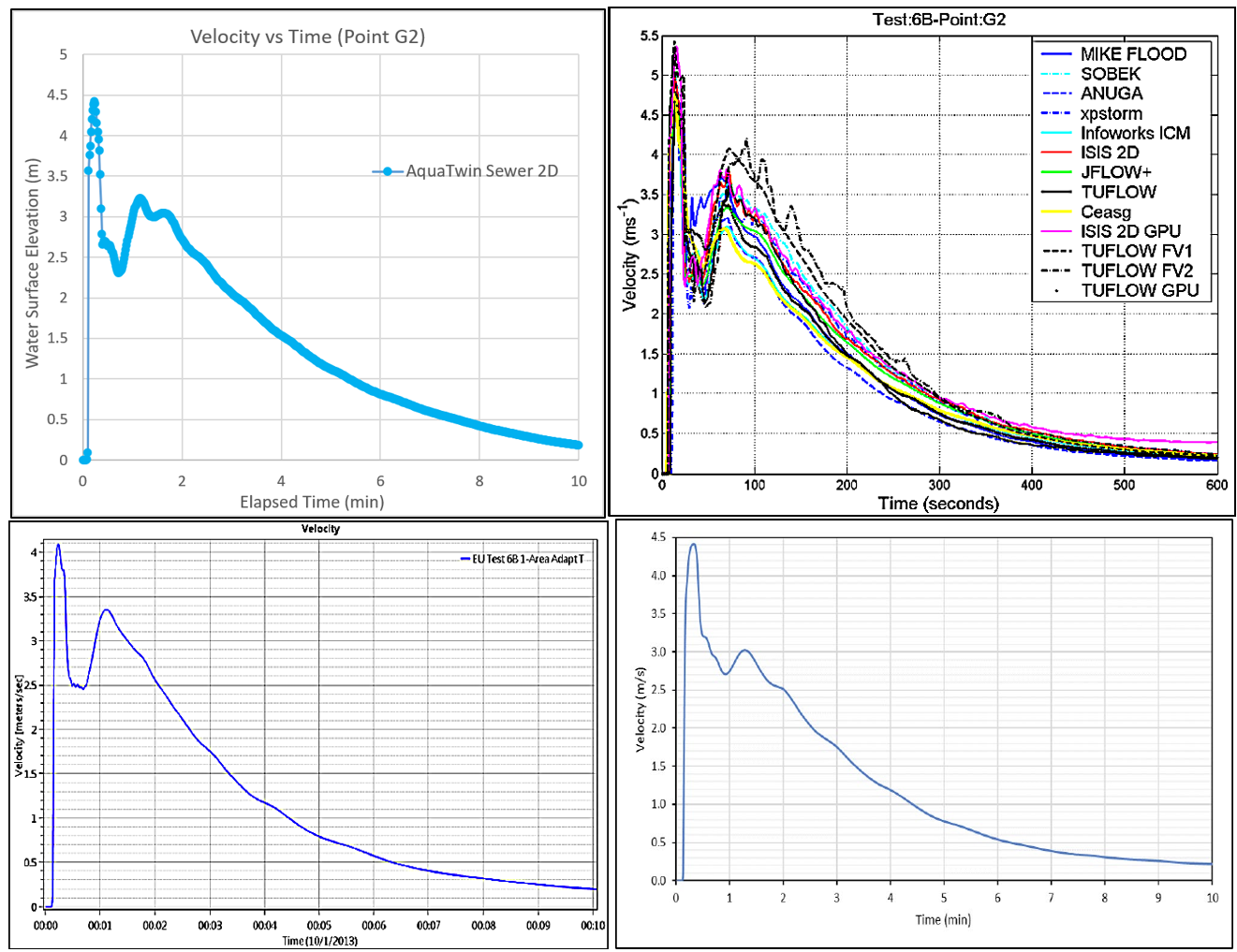
Figure 6B.2) Point G2 Velocity. Top Left: AquaTwin Sewer 2D. Top Right: Ensemble, reproduced from Néelz and Pender (2013); as it appears in Kramer (2021), p. 7-24. Bottom Left: HEC-RAC FEQ, reproduced from Brunner (2018); as it appears in Kramer (2021), p. 7-24. Bottom Right: SRH-2D, reproduced from Kramer (2021), p. 7-24.

Figure 6B.3) Point G4 WSE. Top Left: AquaTwin Sewer 2D. Top Right: Ensemble, reproduced from Néelz and Pender (2013); as it appears in Kramer (2021), p. 7-27. Bottom Left: HEC-RAC FEQ, reproduced from Brunner (2018); as it appears in Kramer (2021), p. 7-27. Bottom Right: SRH-2D, reproduced from Kramer (2021), p. 7-27.

Figure 6B.4) Point G4 Velocity. Top Left: AquaTwin Sewer 2D. Top Right: Ensemble, reproduced from Néelz and Pender (2013); as it appears in Kramer (2021), p. 7-28. Bottom Left: HEC-RAC FEQ, reproduced from Brunner (2018); as it appears in Kramer (2021), p. 7-28. Bottom Right: SRH-2D, reproduced from Kramer (2021), p. 7-28.
Near‑gate gauge (G2): Point G2, immediately downstream of the reservoir gate, again records the passage of the initial gate wave and is the most dynamically demanding of the reported points. AquaTwin predicts the leading edge to arrive within 5 – 10 s, with the WSE rising sharply to an initial shoulder near 2.7 m before settling into an oscillating recession. This arrival timing and peak magnitude track closely with HEC‑RAS (FEQ) and fall within the Ensemble cluster, though slightly underestimating SRH-2D (Fig. 6B.1).
As in Test Case 6A, the sharp initial front is reproduced by the full‑momentum solvers while the recession shows the wider inter‑model scatter characteristic of this location. The velocity time series follows the same pattern seen at Test Case 6A Point G2, a high initial pulse as the gate wave passes, a sharp decline, and a bumpy re‑establishment as the standing jump forms, with AquaTwin’s initial peak velocity of ~4.5 m/s is consistent with SRH‑2D, HEC‑RAS, and the core Ensemble models (Fig. 6B.2).
Wake‑zone gauge (G4): The wake immediately downstream of the obstructing block is the diagnostic location for this test, as it is in Test Case 6A. AquaTwin develops the wake WSE to a peak of ~2.1 m by t ≈ 30 s, followed by a mildly wavy recession as the reservoir drains over the 30-min simulation (10-min shown in Fig. 6B.3).
The peak magnitude and the timing of wake development from AquaTwin agree with SRH‑2D and HEC‑RAS (FEQ) and sit within the Ensemble band throughout; after the initial development it tracks most closely with the full‑momentum packages (TUFLOW and ICM among them), consistent with the Test Case 6A wake‑zone behavior. The corresponding velocity series shows the expected leading pulse and decay, with AquaTwin‘s magnitudes bracketed by SRH‑2D and HEC‑RAS (Fig., 6B.4).
Test Case 8A evaluates a modeling package’s ability to simulate shallow surface inundation in a dense urban catchment (high-resolution), arising from two simultaneous sources: rainfall applied directly to the model grid and a point discharge. The modeled area is an approximately 0.4 km × 1 km section of Glasgow, UK (Cockenzie Street and the surrounding streets), represented by a 0.5 m bare-earth LiDAR Digital Terrain Model with ground elevations ranging from ~21 m to ~37 m (Figure 8A.1). Consistent with the benchmark specification, buildings are omitted and flow is routed over the bare-earth surface.
Inundation is driven by two inputs. The first is a spatially uniform rainfall event applied as rain-on-grid across the modeled area only: a short, high-intensity burst of 400 mm/hr sustained for three minutes (Figure 8A.2). The second is a point source introduced at a single location as the inflow hydrograph in Figure 8A.3. This point source, which represents (for example) culvert overflow, ramps to a peak of 5 m3/s at approximately t = 37 min before receding to zero by t = 55 min. Manning’s roughness is applied to each land use, with n = 0.02 for roads and pavements and n = 0.05 for all other surfaces. All domain boundaries are closed (no flow), and the surface begins dry. The prescribed grid resolution is 2 m (~97,000 computational elements across the 0.4 km2 domain), and the simulation is run for 5 hours to allow the flood to settle in the low-lying parts of the domain.
Relative to the earlier open-terrain tests, Test Case 8A emphasizes very fine mesh resolution, thin sheet flow over complex urban microtopography (curbs, streets, and small depressions), and the interaction of two distinct flood-generation mechanisms — a combination representative of pluvial flooding in a built-up catchment.
Nine output points are distributed across the streets and low-lying areas of the domain (Figure 8A.1). Water surface elevation and velocity are reported at each point at an output interval of 30 s over the 5 hr simulation. Published reference data (Néelz and Pender, 2013) are available at Points 1, 2, 3, and 6 for water surface elevation and at Points 2 and 6 for velocity. Points 2 and 6 are shown and discussed herein, the remaining comparisons with AquaTwin are compiled in Appendix A.8.
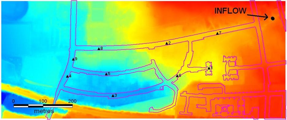
Figure 8A.1. Simulation domain for Test Case 8A with blue-red DEM, sample points, and inflow location.
The DEM (from the UK EA reference documents) was imported into a new AquaTwin project. The road and sample point layers were also provided by the UK EA reference documents. The roads were represented by a land use refinement zone with a Manning’s n = 0.02; the open areas were represented by a default Manning’s n = 0.05. Meshing options were consistent across refinement zones and were calibrated to achieve the recommended grid resolution (~97,000 computational elements). The simulation was run at a 2 s time step; the reporting time was 30 s.
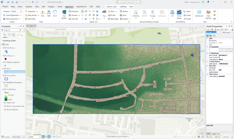
Figure 8A.2. Screenshot of Test Case 8 constructed in the AquaTwin interface.


Figure 8A.3. Spatial extent of Max WSE > 0.2 m for a subset of the simulated domain (bounded by Point 1 on the right, Point 5 on the left). Top: Ensemble, reproduced from Néelz and Pender (2013), p. 104. Bottom: AquaTwin.
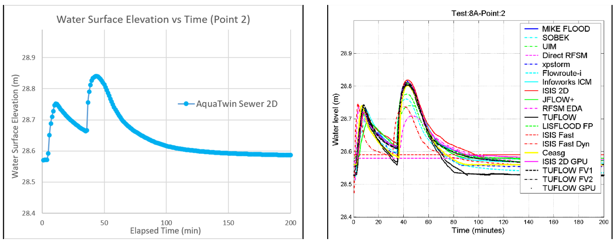
Figure 8A.4. Point 2 WSE. Left: AquaTwin. Right: Ensemble, reproduced from Neelz & Pender, p.101.

Figure 8A.5. Point 6 WSE. Left: AquaTwin. Right: Ensemble, reproduced from Neelz & Pender, p.102.
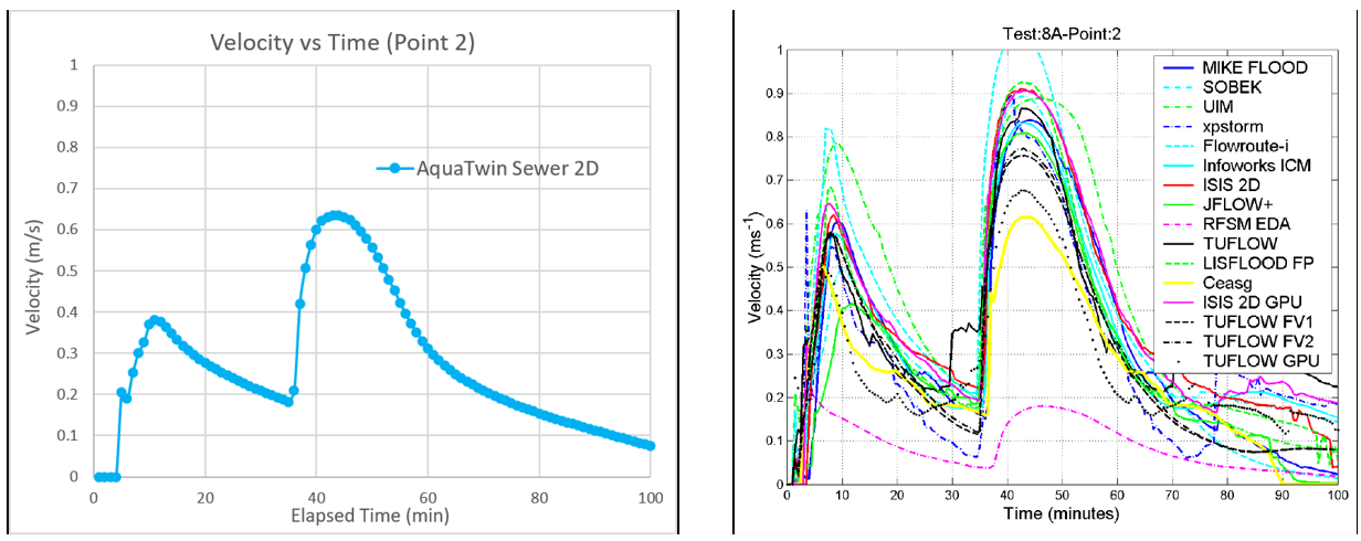
Figure 8A.6. Point 2 Velocity. Left: AquaTwin. Right: Ensemble, reproduced from Neelz & Pender, p.103.
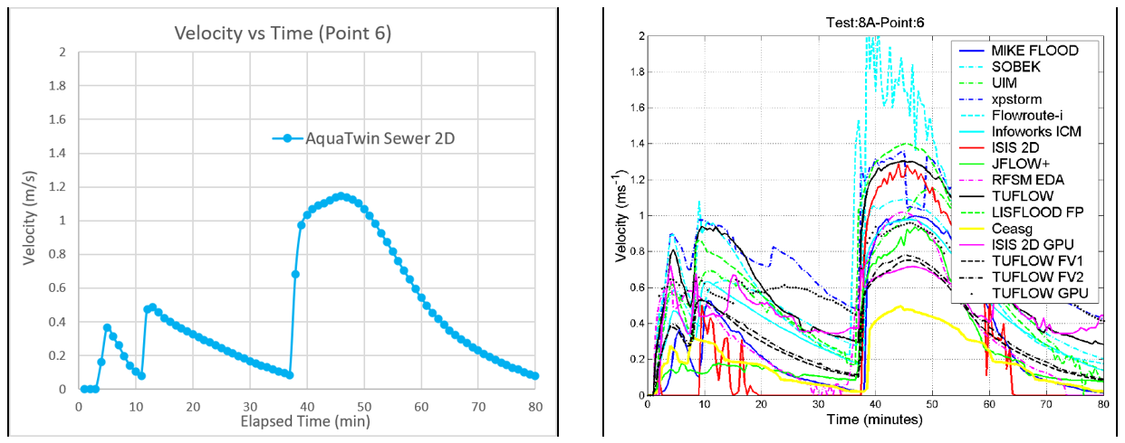
Figure 8A.7. Point 6 Velocity. Left: AquaTwin. Right: Ensemble, reproduced from Neelz & Pender, p.103.
Flood extent: Figure 8A.3 compares the maximum inundation footprint (where max depth >= 0.2 m). AquaTwin’s extent tracks the same connected wet corridors from Point 1 to Point 3, and along the roadway containing Point 2, as the Ensemble models’ inundation map. Spurious wet patches can be seen in AquaTwin, as well as many of the Ensemble models (e.g., ICM, JFLOW+, ISIS 2D GPU, MIKE FLOOD).
WSE: Both Point 2 and Point 6 show a characteristic two-pulse response that reflects the two forcing mechanisms in this test case. A smaller, earlier peak driven by the rainfall burst, followed by a larger peak as the point-source inflow arrives (Figs. 8A.4 & 8A.5). At Point 2, AquaTwin captures this signature cleanly: a first peak of ~28.75 m near t = 8 min, a dip to ~28.66 m, and a principal peak of ~28.84 m at t ≈ 45 min, receding to a ~28.59 m plateau. The shape and timing align closely with the Ensemble, whose main cluster peaks near 28.80 m; AquaTwin sits at the upper edge of that cluster, comparable to ISIS 2D, TUFLOW, MIKE FLOOD, and ICM. At Point 6 the signal is smaller, and the Ensemble spread is wider. AquaTwin’s peak of ~27.06 m is in the upper middle of the Ensemble band, tracking MIKE FLOOD, JFLOW+, and ICM.
Velocity: Velocity is the most scheme-sensitive quantity in this high-resolution urban setting, and the Ensemble spread at Point 2 (Figure 8A.6) is correspondingly the widest of any comparison in the suite. AquaTwin reproduces the same two-pulse velocity structure with correct timing: a first peak of ~0.38 m/s near t = 10 min and a principal peak of ~0.63 m/s at t ≈ 43 min. The magnitudes of velocity fall within the Ensemble band toward its lower edge, near Ceasg and the lower cluster. At Point 6 (Figure 8A.7), a twin-early pulse (t ≈ 5 and 12 min at ~0.4 m/s) is mirrored in timing and shape by the Ensemble main cluster. Similarly, the principal peak of ~1.18 m/s at t ≈ 47 min matches the timing and the centroid of the Ensemble cluster, most like ISIS 2D.
Test Case 8B evaluates a modeling package’s ability to simulate urban surface flooding that originates from a surcharging sewer, i.e., from the coupled 1D-2D exchange between a pressurized underground pipe and the overland surface. It uses the same 0.5 m Glasgow DEM and ~0.4 km2 domain as Test Case 8A, but the flood is generated below ground and emerges at a single manhole (Figure 8B.1). It is the one case in the benchmark suite that exercises coupled 1D–2D behavior directly, and the scenario that most closely mirrors the combined-sewer and stormwater applications for which AquaTwin Sewer 2D is built.
A circular pipe network (1.4 m diameter, 1070 m length, invert set uniformly 2 m below ground elevation) is routed through the 2D domain. All junctions are closed to flooding, except for the manhole (area = 1.0 m2), which is located 467 m downstream of the inflow condition. The outfall is a free surface. The initial condition is 1.6 cms of flow through each conduit. At the upstream junction, an inflow hydrograph is applied, increasing the flow to over 6.2 cms, causing surcharge through the manhole. The surcharged flow is routed onto the overland domain, which is composed of the roadway, buildings, and open areas.
The roughness (n = 0.02 for roads and pavements, 0.05 elsewhere), 2 m grid resolution (~97,000 elements), closed outer boundaries, dry initial surface, and 5 hr run time are identical to Test Case 8A. The defining challenge of Test Case 8B is therefore not the surface hydraulics alone but the fidelity of the 1D–2D coupling: the volume and timing of the manhole surcharge, and the redistribution of that volume across a building-constrained urban surface.
Water surface elevation and velocity are reported at the domain’s output points (Figure 8B.1), together with the discharge through the surcharging manhole, at an output interval of 30 s over the 5 hr simulation. Published reference data (Néelz and Pender, 2013) are available at Points 1, 2, and 3 for WSE and at Point 3 for velocity.
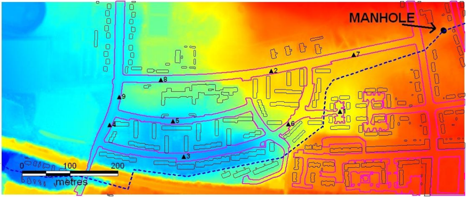
Figure 8B.1. Simulation domain for Test Case 8B with blue-red DEM, sample points, and surcharge location. Inflow condition is from the right; outflow condition is to the left.
The DEM (from the UK EA reference documents) was imported into a new AquaTwin project. The road, building, and sample point layers were also provided by the UK EA reference documents. The roads were represented by a land use refinement zone with a Manning’s n = 0.02; buildings were also represented by a land use refinement zone with a 10 m elevation offset; the open areas were represented by a default Manning’s n = 0.05. Meshing options were consistent across refinement zones and were calibrated to achieve the recommended grid resolution (~97,000 computational elements). The simulation was run at a 2 s time step; the reporting time was 30 s for a 5-hr simulation duration.

Figure 8B.2. Screenshot of Test Case 8B constructed in AquaTwin. 2D simulation domain contains ~92,000 triangular mesh elements; buildings (beige) and roadway (grey) layers are visible. 1D network is seen to follow roughly the Camlachie Burn waterway with inflow and outfall outside the 2D domain.

Figure 8B.3. Plan view of Worst Case WSE for northeast corner of simulation domain. Surcharging manhole is in the top right; Point 2 is to the left; Point 6 is on the bottom left.
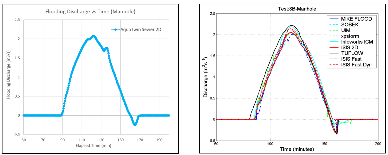
Figure 8B.4. Manhole Flooding. Left: AquaTwin. Right: Ensemble, reproduced from Neelz & Pender, p.110.

Table 8B.1. Manhole Flooding Volumes, reproduced from Neelz & Pender, p.110.

Figure 8B.5. Point 1 WSE. Left: AquaTwin. Right: Ensemble, reproduced from Neelz & Pender, p.111.
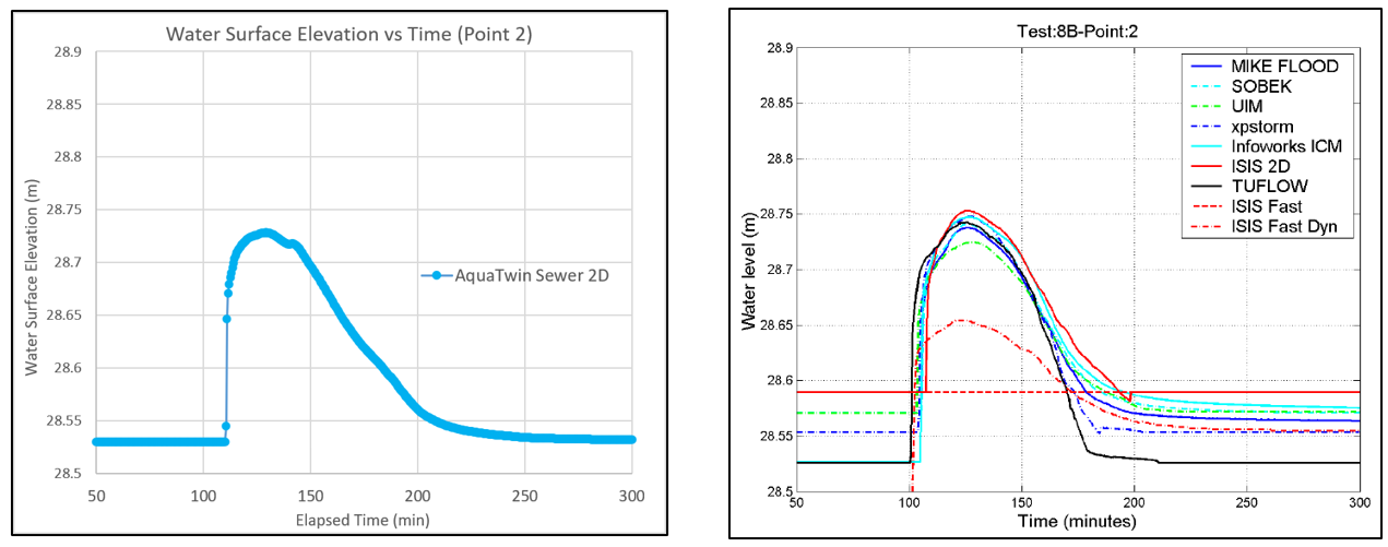
Figure 8B.6. Point 2 WSE. Left: AquaTwin. Right: Ensemble, reproduced from Neelz & Pender, p.111.
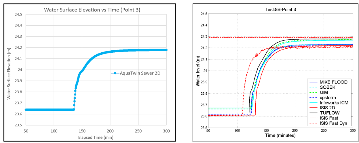
Figure 8B.7. Point 3 WSE. Left: AquaTwin. Right: Ensemble, reproduced from Neelz & Pender, p.112.
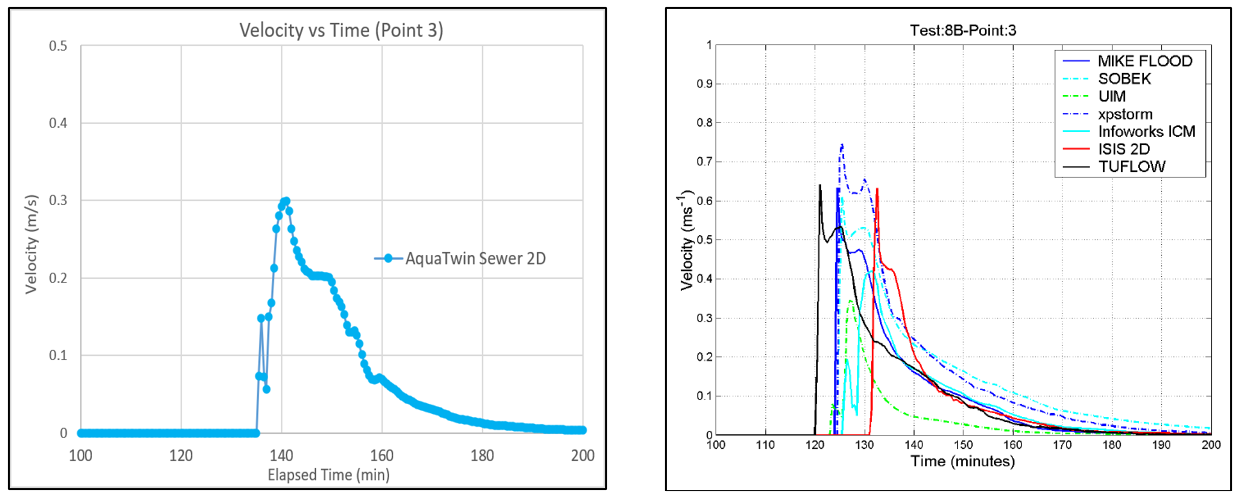
Figure 8B.8. Point 3 Velocity. Left: AquaTwin. Right: Ensemble, reproduced from Neelz & Pender, p.112.
Manhole Surcharge: The defining quantity for Test Case 8B is the exchange between the 1D network and the 2D overland surface. The manhole flooding hydrograph (Figure 8B.4.) begins around t = 90 min, peaks at ~2.1 cms near t = 120 min, and recedes back to zero by t = 160 min. After the main hydrograph, there is a brief period of negative flooding, which indicates that the model is capable of bidirectional exchange between the 1D network and 2D overland surface. AquaTwin performs convincingly; the total manhole flood volume of 5,360 m3 (Table 8B.1) falls squarely within the Ensemble range, as do the peak and negative flow hydrographs.
WSE: Due to the single forcing mechanism in this test case, the manhole surcharge, the WSE at Points 1 & 2 exhibit a single pulse (Figs 8B.5 & 8B.6), in contrast to the two-pulse response in Test Case 8A. At Point 1, AquaTwin holds the ~27.1 m baseline until the surcharge arrives near t = 115 min, rises to a peak of ~27.62 m, and settles to a ~27.52 m plateau — coincident with the reference cluster in both magnitude and timing. At Point 2, AquaTwin peaks at ~28.73 m near t = 127 min, in the heart of the ensemble cluster (~28.72–28.75 m), before receding to a ~28.53 m plateau at the lower edge of the reference band. Point 3, farthest into the domain, fills gradually rather than as a sharp pulse; AquaTwin captures this S-shaped rise and settles at ~24.17 m, marginally (~0.03–0.05 m) below the ensemble plateau of ~24.20–24.25 m, with an arrival a few minutes later than the reference median. Across all three points the form, timing, and settled levels are consistent with the established solvers.
This study applied AquaTwin Sewer 2D (Aquanuity) to the full nine-case UK Environment Agency (UK EA) 2D benchmark suite and evaluated its predictions against 21 reference models: the 19-industry simulation package ensemble of Néelz and Pender (2013) together with datasets from HEC-RAS 2D (Brunner, 2018) and SRH-2D (Kramer, 2021). The suite was chosen because its cases isolate distinct physical behaviors: mass conservation and wetting/drying (Test Case 1), low-momentum depression filling (Test Case 2), momentum conservation over an obstruction (Test Case 3), flood-wave celerity across an open floodplain (Test Case 4), transcritical valley inundation from a dam failure (Test Case 5), laboratory- and field-scale dam breaks with hydraulic jumps and building wakes (Test Cases 6A and 6B), and high-resolution urban rainfall, point-source, and surcharge flow (Test Cases 8A and 8B). Across the nine test cases, AquaTwin was evaluated at 51 distinct sample locations, comprising 83 individual water-surface-elevation and velocity time-series comparisons.
A central, and expected, finding is that the 21 reference models do not agree perfectly with one another. This inter-model spread is itself a working measure of the engineering uncertainty inherent in 2D hydraulic modeling, and it is not constant: it is narrow for the simplest cases and widens systematically as the physics become more demanding. Another landmark finding is that AquaTwin is within the engineering uncertainty on 83 out of 83 individual test-point pairs, and clustered within the central band of full-SWE solvers in the majority.
In Test Cases 1 – 4, the reference model ensemble, including HEC-RAS and SRH-2D, is effectively a single curve, from which AquaTwin is indistinguishable. As the cases add data structures, higher-resolution meshes, and transcritical transitions (Tests 5 and 6), the ensemble fans out, with several well-known packages appearing at the margins of the band. At every one of these documented sample points, AquaTwin fell within the ensemble band. Stated formally, for each reported quantity x the AquaTwin prediction satisfied xmin ≤ xAquaTwin ≤ xmax relative to the reference set, and it typically sat near the ensemble central tendency rather than at its edges. The central tendency was largely defined by other full-SWE models, listed in Table 1.
AquaTwin held this position without any loss of stability in the most dynamic cases. In the Test Case 5 dam-break wave and the Test Case 6A laboratory flume (where flow arrivals are abrupt and hydraulic jumps stand and oscillate) AquaTwin reproduced sharp wave-front arrivals, peak magnitudes, and recession limbs cleanly, avoiding the numerical oscillation and instability that pushed some ensemble members toward the outer edges of the spread. Test Case 6A is also the one case in the suite with physical measurements, taken from the UCL flume; there, AquaTwin’s reservoir drawdown, wake-zone peak, and near-gate spike timing tracked the observed data, not merely the numerical consensus.
Taken together, the benchmark comparisons summarized here show that AquaTwin performs on par with the established full-SWE packages across the full range of regimes tested within the UK EA benchmarking suite.
Aquanuity, Inc. (2026). AquaTwin Sewer Help Documentation. Version 2.6. Accessed May 2026. https://aquanuity.com/aquatwinhelp/sewer
Brunner, G.W. (2018). Benchmarking of the HEC-RAS Two-Dimensional Hydraulic Modeling Capabilities. RD-51. U.S. Army Corps of Engineers, Hydrologic Engineering Center, Davis, CA.
Brunner, G.W. (2021). HEC-RAS 2D Modeling User’s Manual, Version 6.0. CPD-68A. U.S. Army Corps of Engineers, Hydrologic Engineering Center, Davis, CA.
Kramer, C. (2021). Benchmarking of SRH-2D. Publication No. FHWA-RC-21-0006. Federal Highway Administration, Office of Infrastructure Research and Development, McLean, VA
Lai, Y.G. (2008). SRH-2D Version 2: Theory and User’s Manual. U.S. Bureau of Reclamation, Technical Service Center, Denver, CO.
Néelz, S., and G. Pender (2010). Benchmarking of 2D Hydraulic Modelling Packages. Environment Agency Science Report SC080035/SR2, Environment Agency, Bristol, UK.
Soares-Frazão, S. and Zech, Y. (2002). Dambreak flow experiment: the isolated building test case. Technical Report, WP3 Flood Propagation, IMPACT (Investigation of Extreme Flood Processes and Uncertainty), EC Research Project No. EVG1-CT2001-0037. Available from: http://www.impact-project.net/wp3_technical.htm
Vreugdenhil, C.B. (1994). Numerical Methods for Shallow-Water Flow. Water Science and Technology Library, Vol. 13. Kluwer Academic Publishers, Dordrecht, The Netherlands. ISBN 978-0-7923-3164-3.
This appendix contains the full suite of AquaTwin and previously published WSE and velocity figures for all sample points for all test cases. For more information about the setup for each test case and a discussion of the agreement between each subfigure, see the main report. To reduce the page count of the main report, only a subset of sample points were included therein.
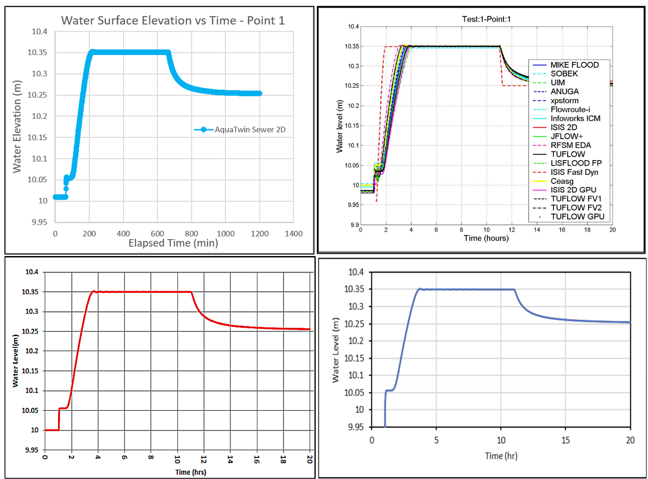
Figure A1.1) Point 1 WSE. Top left: AquaTwin. Top right: Ensemble, reproduced from Néelz and Pender (2013); as it appears in Kramer (2021), p. 2-4. Bottom left: HEC-RAS, reproduced from Brunner (2018); as it appears in Kramer (2021), p. 2-4. Bottom right: SRH-2D, reproduced from Kramer (2021), p. 2-4.
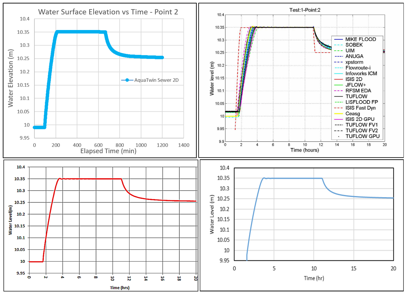
Figure A1.2) Point 2 WSE. Top left: AquaTwin. Top right: Ensemble, reproduced from Néelz and Pender (2013); as it appears in Kramer (2021), p. 2-5. Bottom left: HEC-RAS, reproduced from Brunner (2018); as it appears in Kramer (2021), p. 2-5. Bottom right: SRH-2D, reproduced from Kramer (2021), p. 2-5.

Figure A2.1) Point 1 WSE. Top left: AquaTwin. Top right: Ensemble, reproduced from Néelz and Pender (2013); as it appears in Kramer (2021), p. 3-9. Bottom left: HEC-RAS, reproduced from Brunner (2018); as it appears in Kramer (2021), p. 3-9. Bottom right: SRH-2D, reproduced from Kramer (2021), p. 3-9.
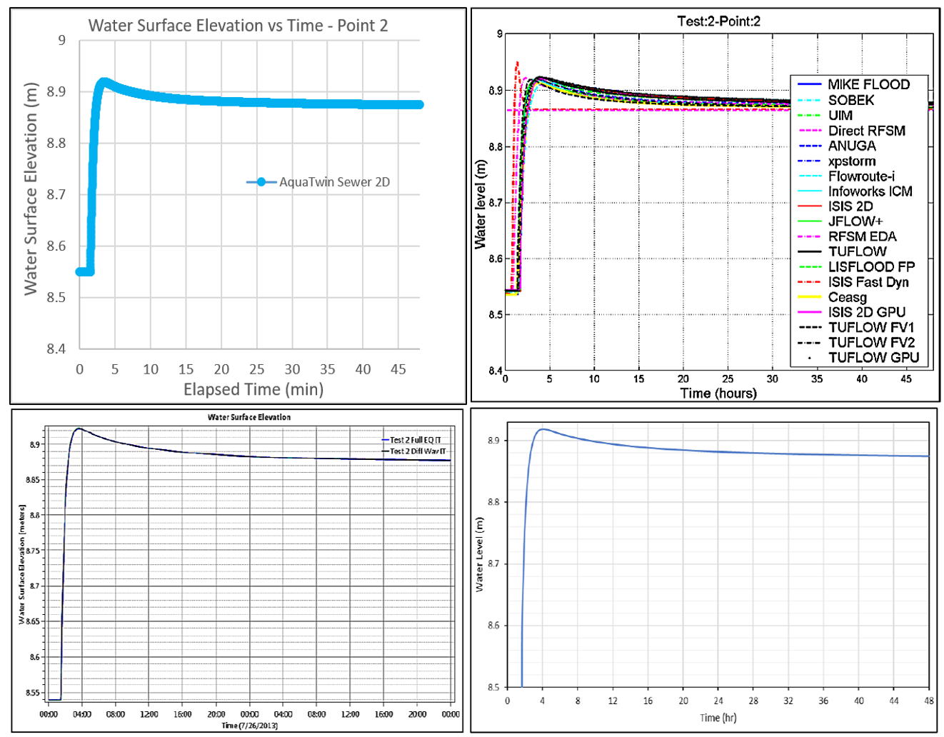
Figure A2.2) Point 2 WSE. Top left: AquaTwin. Top right: Ensemble, reproduced from Néelz and Pender (2013); as it appears in Kramer (2021), p. 3-8. Bottom left: HEC-RAS, reproduced from Brunner (2018); as it appears in Kramer (2021), p. 3-8. Bottom right: SRH-2D, reproduced from Kramer (2021), p. 3-8.

Figure A2.3) Point 3 WSE. Top left: AquaTwin. Top right: Ensemble, reproduced from Néelz and Pender (2013); as it appears in Kramer (2021), p. 3-7. Bottom left: HEC-RAS, reproduced from Brunner (2018); as it appears in Kramer (2021), p. 3-7. Bottom right: SRH-2D, reproduced from Kramer (2021), p. 3-7.
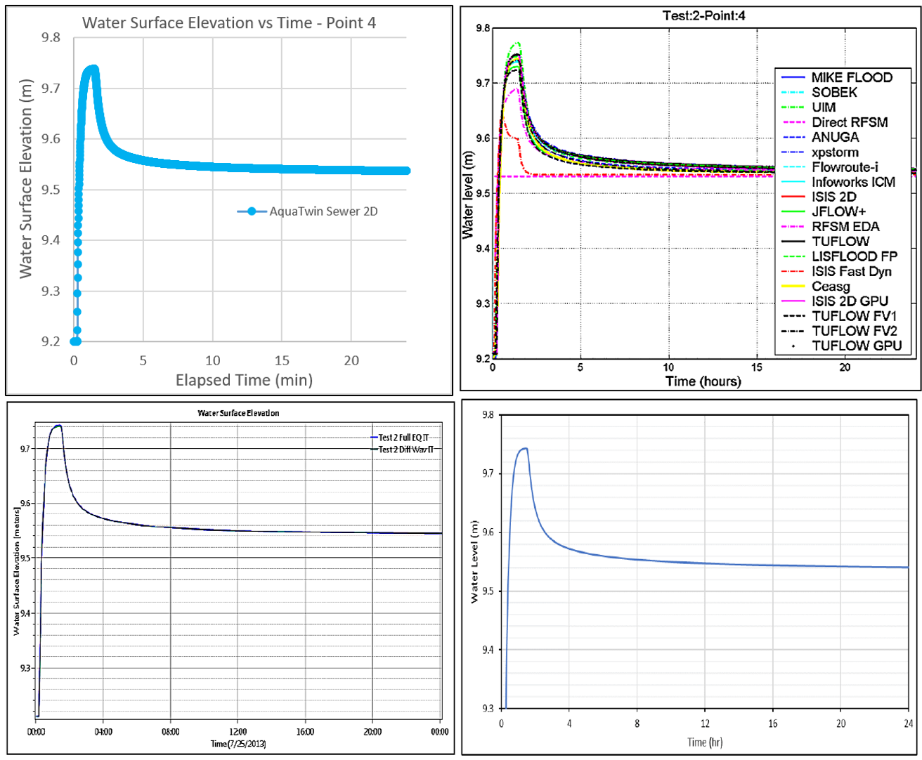
Figure A2.4) Point 4 WSE. Top left: AquaTwin. Top right: Ensemble, reproduced from Néelz and Pender (2013); as it appears in Kramer (2021), p. 3-6. Bottom left: HEC-RAS, reproduced from Brunner (2018); as it appears in Kramer (2021), p. 3-6. Bottom right: SRH-2D, reproduced from Kramer (2021), p. 3-6.

Figure A2.5) Point 5 WSE. Top left: AquaTwin. Top right: Ensemble, reproduced from Néelz and Pender (2013); as it appears in Kramer (2021), p. 3-13. Bottom left: HEC-RAS, reproduced from Brunner (2018); as it appears in Kramer (2021), p. 3-13. Bottom right: SRH-2D, reproduced from Kramer (2021), p. 3-13.

Figure A2.6) Point 6 WSE. Top left: AquaTwin. Top right: Ensemble, reproduced from Néelz and Pender (2013); as it appears in Kramer (2021), p. 3-12. Bottom left: HEC-RAS, reproduced from Brunner (2018); as it appears in Kramer (2021), p. 3-12. Bottom right: SRH-2D, reproduced from Kramer (2021), p. 3-12.

Figure A2.7) Point 7 WSE. Top left: AquaTwin. Top right: Ensemble, reproduced from Néelz and Pender (2013); as it appears in Kramer (2021), p. 3-11. Bottom left: HEC-RAS, reproduced from Brunner (2018); as it appears in Kramer (2021), p. 3-11. Bottom right: SRH-2D, reproduced from Kramer (2021), p. 3-11.

Figure A2.8) Point 8 WSE. Top left: AquaTwin. Top right: Ensemble, reproduced from Néelz and Pender (2013); as it appears in Kramer (2021), p. 3-10. Bottom left: HEC-RAS, reproduced from Brunner (2018); as it appears in Kramer (2021), p. 3-10. Bottom right: SRH-2D, reproduced from Kramer (2021), p. 3-10.
**Sample Point 9 was dry and not reported in any of the reference reports.

Figure A2.9) Point 10 WSE. Top left: AquaTwin. Top right: Ensemble, reproduced from Néelz and Pender (2013); as it appears in Kramer (2021), p. 3-16. Bottom left: HEC-RAS, reproduced from Brunner (2018); as it appears in Kramer (2021), p. 3-16. Bottom right: SRH-2D, reproduced from Kramer (2021), p. 3-16.

Figure A2.10) Point 11 WSE. Top left: AquaTwin. Top right: Ensemble, reproduced from Néelz and Pender (2013); as it appears in Kramer (2021), p. 3-15. Bottom left: HEC-RAS, reproduced from Brunner (2018); as it appears in Kramer (2021), p. 3-15. Bottom right: SRH-2D, reproduced from Kramer (2021), p. 3-15.

Figure A2.11) Point 12 WSE. Top left: AquaTwin. Top right: Ensemble, reproduced from Néelz and Pender (2013); as it appears in Kramer (2021), p. 3-14. Bottom left: HEC-RAS, reproduced from Brunner (2018); as it appears in Kramer (2021), p. 3-14. Bottom right: SRH-2D, reproduced from Kramer (2021), p. 3-14.
**Sample Points 13 – 16 were dry and not reported in any of the reference reports.

Figure A3.1) Point 1 WSE. Top left: AquaTwin. Top right: Ensemble, reproduced from Néelz and Pender (2013); as it appears in Kramer (2021), p. 4-5. Bottom left: HEC-RAS, reproduced from Brunner (2018); as it appears in Kramer (2021), p. 4-5. Bottom right: SRH-2D, reproduced from Kramer (2021), p. 4-5.
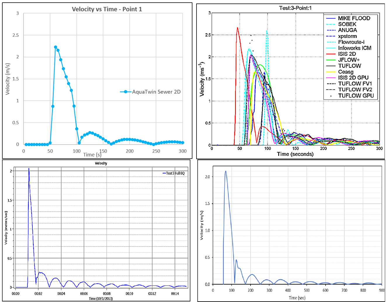
Figure A3.2) Point 1 Water Velocity. Top left: AquaTwin. Top right: Ensemble, reproduced from Néelz and Pender (2013); as it appears in Kramer (2021), p. 4-6. Bottom left: HEC-RAS, reproduced from Brunner (2018); as it appears in Kramer (2021), p. 4-6. Bottom right: SRH-2D, reproduced from Kramer (2021), p. 4-6.
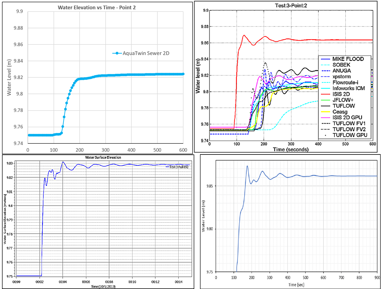
Figure A3.3) Point 2 WSE. Top left: AquaTwin. Top right: Ensemble, reproduced from Néelz and Pender (2013); as it appears in Kramer (2021), p. 4-7. Bottom left: HEC-RAS, reproduced from Brunner (2018); as it appears in Kramer (2021), p. 4-7. Bottom right: SRH-2D, reproduced from Kramer (2021), p. 4-7.

Figure A3.4) Point 2 Water Velocity. Top left: AquaTwin. Bottom left: HEC-RAS, reproduced from Brunner (2018); as it appears in Kramer (2021), p. 4-8. Bottom right: SRH-2D, reproduced from Kramer (2021), p. 4-8.

Figure A4.1) Point 1 WSE. Top left: AquaTwin. Top right: Ensemble, reproduced from Néelz and Pender (2013); as it appears in Kramer (2021), p. 5-6. Bottom left: HEC-RAS, reproduced from Brunner (2018); as it appears in Kramer (2021), p. 5-6. Bottom right: SRH-2D, reproduced from Kramer (2021), p. 5-6.
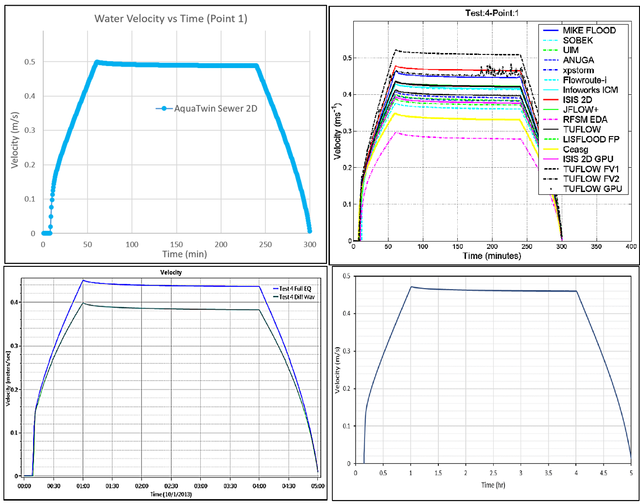
Figure A4.2) Point 1 Water Velocity. Top left: AquaTwin. Top right: Ensemble, reproduced from Néelz and Pender (2013); as it appears in Kramer (2021), p. 5-7. Bottom left: HEC-RAS, reproduced from Brunner (2018); as it appears in Kramer (2021), p. 5-7. Bottom right: SRH-2D, reproduced from Kramer (2021), p. 5-7.
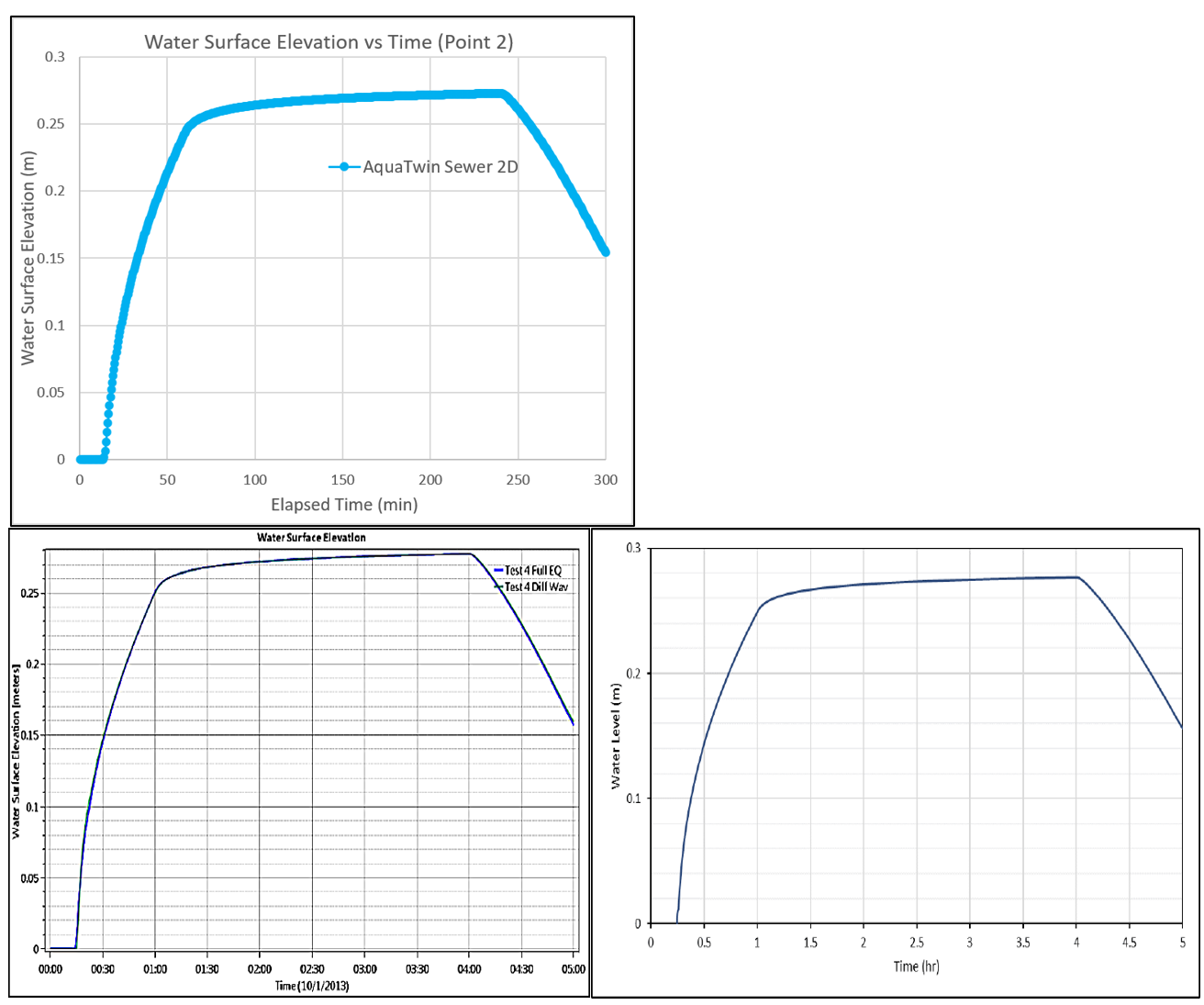
Figure A4.3) Point 2 WSE. Top left: AquaTwin. Bottom left: HEC-RAS, reproduced from Brunner (2018); as it appears in Kramer (2021), p. 5-8. Bottom right: SRH-2D, reproduced from Kramer (2021), p. 5-8.
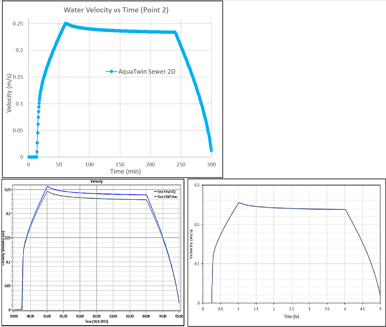
Figure A4.4) Point 2 Water Velocity. Top left: AquaTwin. Bottom left: HEC-RAS, reproduced from Brunner (2018); as it appears in Kramer (2021), p. 5-9. Bottom right: SRH-2D, reproduced from Kramer (2021), p. 5-9.

Figure A4.5) Point 3 WSE. Top left: AquaTwin. Top right: Ensemble, reproduced from Néelz and Pender (2013); as it appears in Kramer (2021), p. 5-10. Bottom left: HEC-RAS, reproduced from Brunner (2018); as it appears in Kramer (2021), p. 5-10. Bottom right: SRH-2D, reproduced from Kramer (2021), p. 5-10.
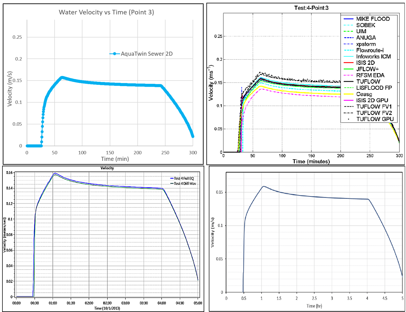
Figure A4.6) Point 3 Water Velocity. Top left: AquaTwin. Top right: Ensemble, reproduced from Néelz and Pender (2013); as it appears in Kramer (2021), p. 5-11. Bottom left: HEC-RAS, reproduced from Brunner (2018); as it appears in Kramer (2021), p. 5-11. Bottom right: SRH-2D, reproduced from Kramer (2021), p. 5-11.
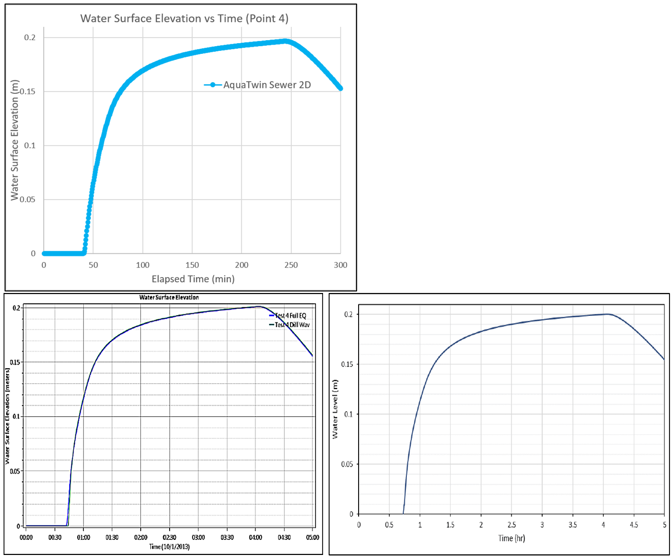
Figure A4.7) Point 4 WSE. Top left: AquaTwin. Bottom left: HEC-RAS, reproduced from Brunner (2018); as it appears in Kramer (2021), p. 5-12. Bottom right: SRH-2D, reproduced from Kramer (2021), p. 5-12.
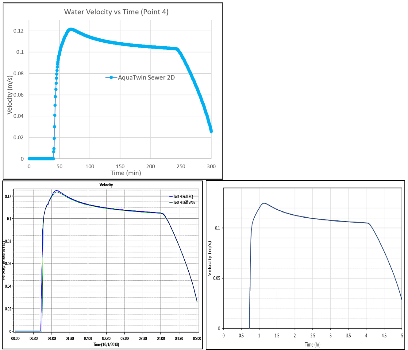
Figure A4.8) Point 4 Water Velocity. Top left: AquaTwin. Bottom left: HEC-RAS, reproduced from Brunner (2018); as it appears in Kramer (2021), p. 5-13. Bottom right: SRH-2D, reproduced from Kramer (2021), p. 5-13.

Figure A4.9) Point 5 WSE. Top left: AquaTwin. Top right: Ensemble, reproduced from Néelz and Pender (2013); as it appears in Kramer (2021), p. 5-14. Bottom left: HEC-RAS, reproduced from Brunner (2018); as it appears in Kramer (2021), p. 5-14. Bottom right: SRH-2D, reproduced from Kramer (2021), p. 5-14.
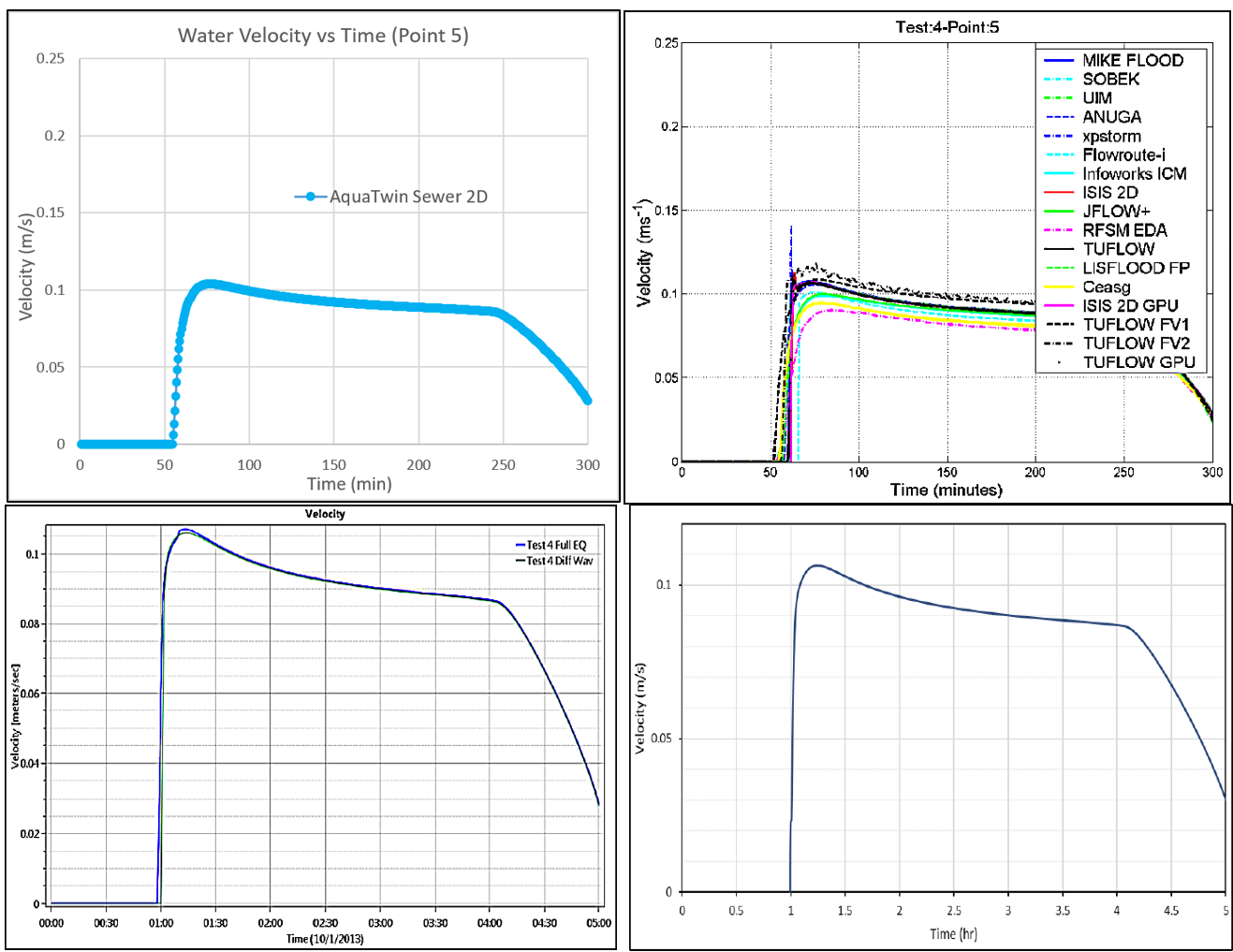
Figure A4.10) Point 5 Water Velocity. Top left: AquaTwin. Top right: Ensemble, reproduced from Néelz and Pender (2013); as it appears in Kramer (2021), p. 5-15. Bottom left: HEC-RAS, reproduced from Brunner (2018); as it appears in Kramer (2021), p. 5-15. Bottom right: SRH-2D, reproduced from Kramer (2021), p. 5-15.
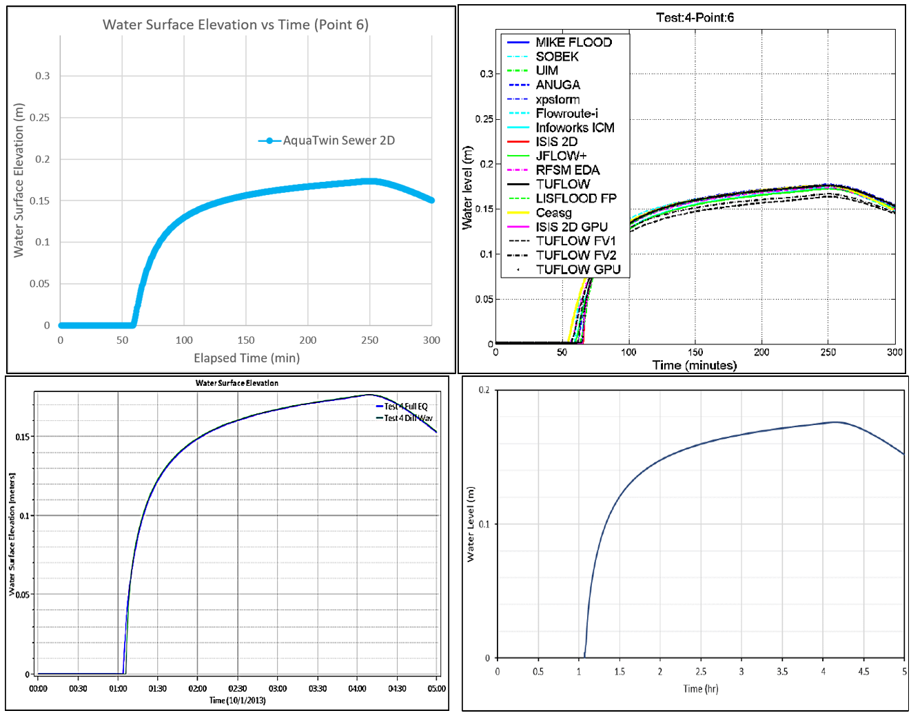
Figure A4.11) Point 6 WSE. Top left: AquaTwin. Top right: Ensemble, reproduced from Néelz and Pender (2013); as it appears in Kramer (2021), p. 5-16. Bottom left: HEC-RAS, reproduced from Brunner (2018); as it appears in Kramer (2021), p. 5-16. Bottom right: SRH-2D, reproduced from Kramer (2021), p. 5-16.
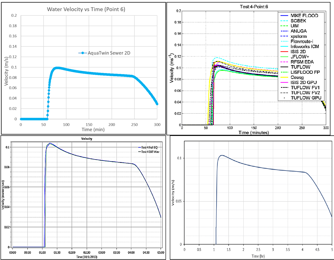
Figure A4.12) Point 6 Water Velocity. Top left: AquaTwin. Top right: Ensemble, reproduced from Néelz and Pender (2013); as it appears in Kramer (2021), p. 5-17. Bottom left: HEC-RAS, reproduced from Brunner (2018); as it appears in Kramer (2021), p. 5-17. Bottom right: SRH-2D, reproduced from Kramer (2021), p. 5-17.

Figure A5.1) Point 1 WSE. Top left: AquaTwin. Top right: Ensemble, reproduced from Néelz and Pender (2013); as it appears in Kramer (2021), p. 6-5. Bottom left: HEC-RAS, reproduced from Brunner (2018); as it appears in Kramer (2021), p. 6-5. Bottom right: SRH-2D, reproduced from Kramer (2021), p. 6-5.

Figure A5.2) Point 1 Magnitude of Water Velocity. Top left: AquaTwin. Top right: Ensemble, reproduced from Néelz and Pender (2013); as it appears in Kramer (2021), p. 6-6. Bottom left: HEC-RAS, reproduced from Brunner (2018); as it appears in Kramer (2021), p. 6-6. Bottom right: SRH-2D, reproduced from Kramer (2021), p. 6-6.

Figure A5.3) Point 2 WSE. Top left: AquaTwin. Bottom left: HEC-RAS, reproduced from Brunner (2018); as it appears in Kramer (2021), p. 6-7. Bottom right: SRH-2D, reproduced from Kramer (2021), p. 6-7.

Figure A5.4) Point 2 Magnitude of Water Velocity. Top left: AquaTwin. Bottom left: HEC-RAS, reproduced from Brunner (2018); as it appears in Kramer (2021), p. 6-8. Bottom right: SRH-2D, reproduced from Kramer (2021), p. 6-8.

Figure A5.5) Point 3 WSE. Top left: AquaTwin. Top right: Ensemble, reproduced from Néelz and Pender (2013); as it appears in Kramer (2021), p. 6-9. Bottom left: HEC-RAS, reproduced from Brunner (2018); as it appears in Kramer (2021), p. 6-9. Bottom right: SRH-2D, reproduced from Kramer (2021), p. 6-9.

Figure A5.6) Point 3 Magnitude of Water Velocity. Top left: AquaTwin. Top right: Ensemble, reproduced from Néelz and Pender (2013); as it appears in Kramer (2021), p. 6-10. Bottom left: HEC-RAS, reproduced from Brunner (2018); as it appears in Kramer (2021), p. 6-10. Bottom right: SRH-2D, reproduced from Kramer (2021), p. 6-10.
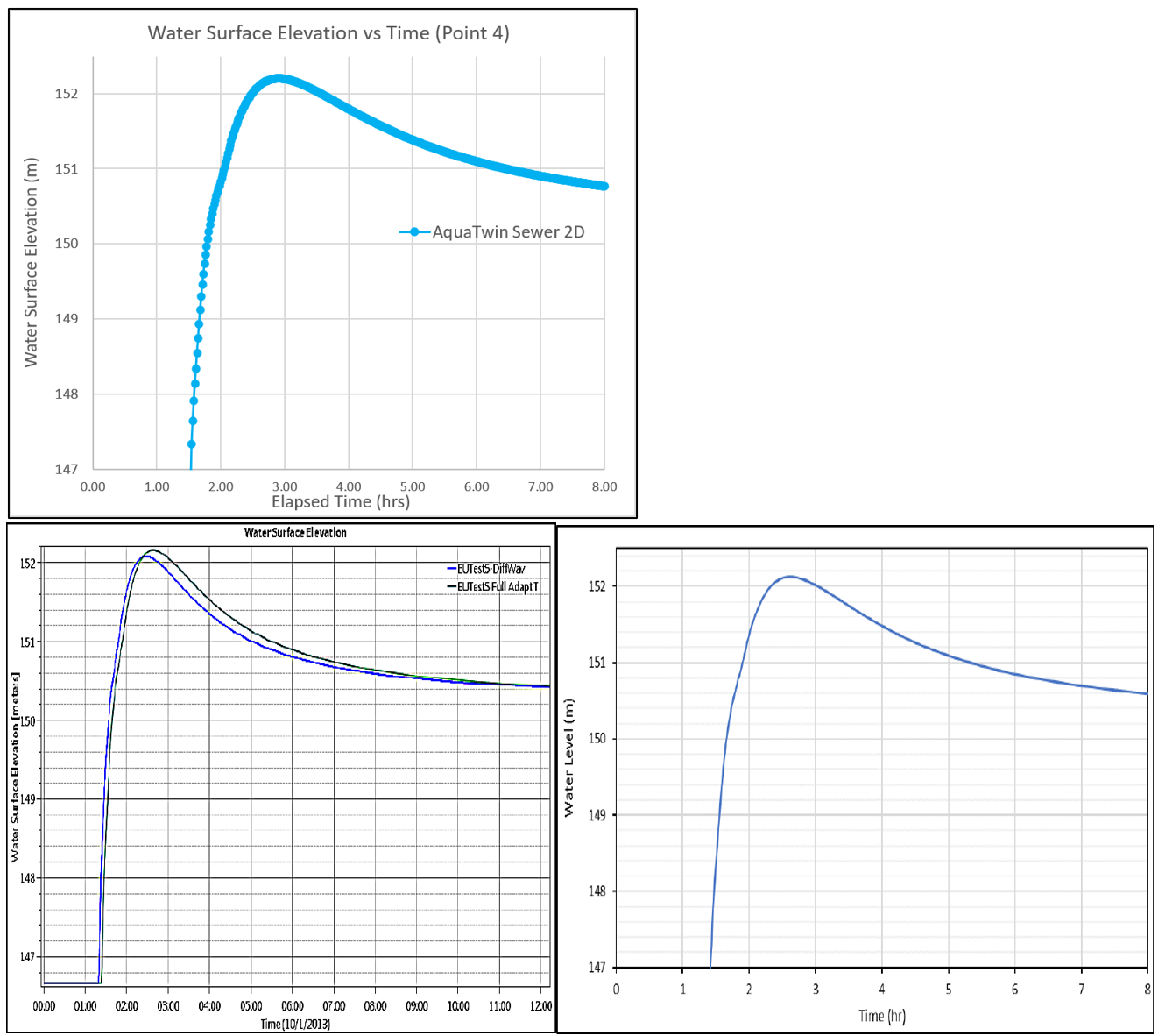
Figure A5.7) Point 4 WSE. Top left: AquaTwin. Bottom left: HEC-RAS, reproduced from Brunner (2018); as it appears in Kramer (2021), p. 6-11. Bottom right: SRH-2D, reproduced from Kramer (2021), p. 6-11.

Figure A5.8) Point 4 Magnitude of Water Velocity. Top left: AquaTwin. Top right: Ensemble, reproduced from Néelz and Pender (2013); as it appears in Kramer (2021), p. 6-12. Bottom left: HEC-RAS, reproduced from Brunner (2018); as it appears in Kramer (2021), p. 6-12. Bottom right: SRH-2D, reproduced from Kramer (2021), p. 6-12.

Figure A5.9) Point 5 WSE. Top left: AquaTwin. Top right: Ensemble, reproduced from Néelz and Pender (2013); as it appears in Kramer (2021), p. 6-13. Bottom left: HEC-RAS, reproduced from Brunner (2018); as it appears in Kramer (2021), p. 6-13. Bottom right: SRH-2D, reproduced from Kramer (2021), p. 6-13.

Figure A5.10) Point 5 Water Velocity. Top left: AquaTwin. Bottom left: HEC-RAS, reproduced from Brunner (2018); as it appears in Kramer (2021), p. 6-14. Bottom right: SRH-2D, reproduced from Kramer (2021), p. 6-14.
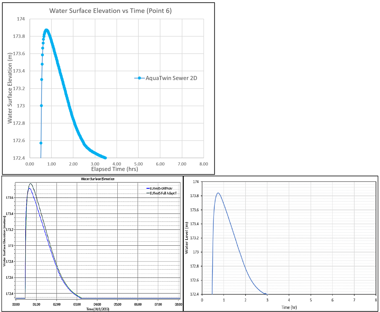
Figure A5.11) Point 6 WSE. Top left: AquaTwin. Bottom left: HEC-RAS, reproduced from Brunner (2018); as it appears in Kramer (2021), p. 6-15. Bottom right: SRH-2D, reproduced from Kramer (2021), p. 6-15.
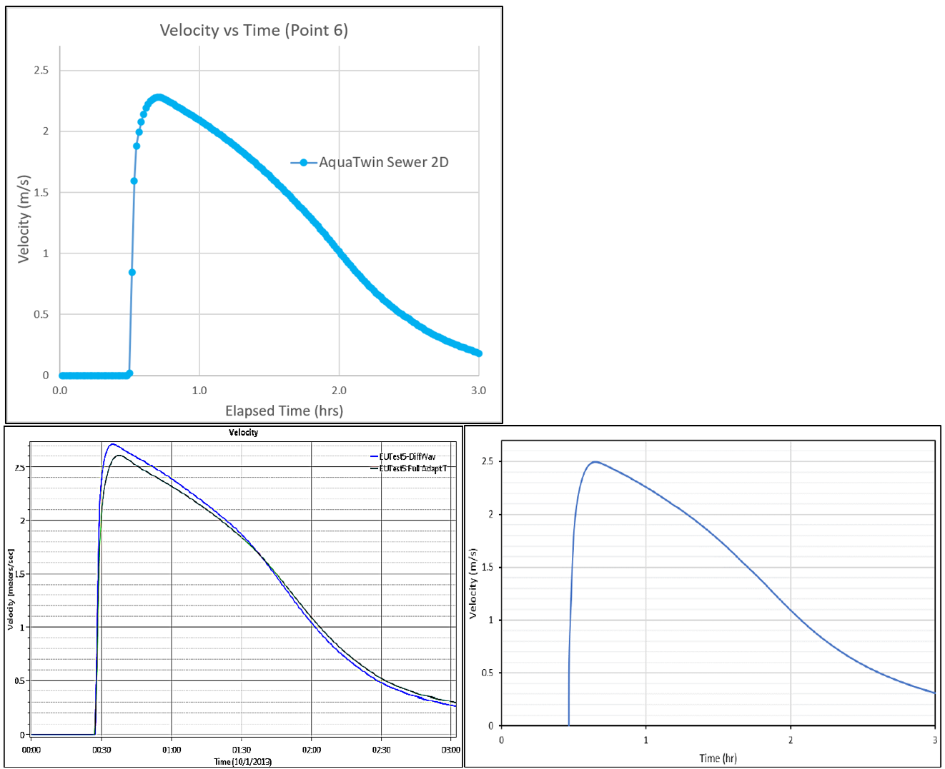
Figure A5.12) Point 6 Water Velocity. Top left: AquaTwin. Bottom left: HEC-RAS, reproduced from Brunner (2018); as it appears in Kramer (2021), p. 6-16. Bottom right: SRH-2D, reproduced from Kramer (2021), p. 6-16.

Figure A5.13) Point 7 WSE. Top left: AquaTwin. Top right: Ensemble, reproduced from Néelz and Pender (2013); as it appears in Kramer (2021), p. 6-17. Bottom left: HEC-RAS, reproduced from Brunner (2018); as it appears in Kramer (2021), p. 6-17. Bottom right: SRH-2D, reproduced from Kramer (2021), p. 6-17.

Figure A5.14) Point 7 Water Velocity. Top left: AquaTwin. Top right: Ensemble, reproduced from Néelz and Pender (2013); as it appears in Kramer (2021), p. 6-18. Bottom left: HEC-RAS, reproduced from Brunner (2018); as it appears in Kramer (2021), p. 6-18. Bottom right: SRH-2D, reproduced from Kramer (2021), p. 6-18.
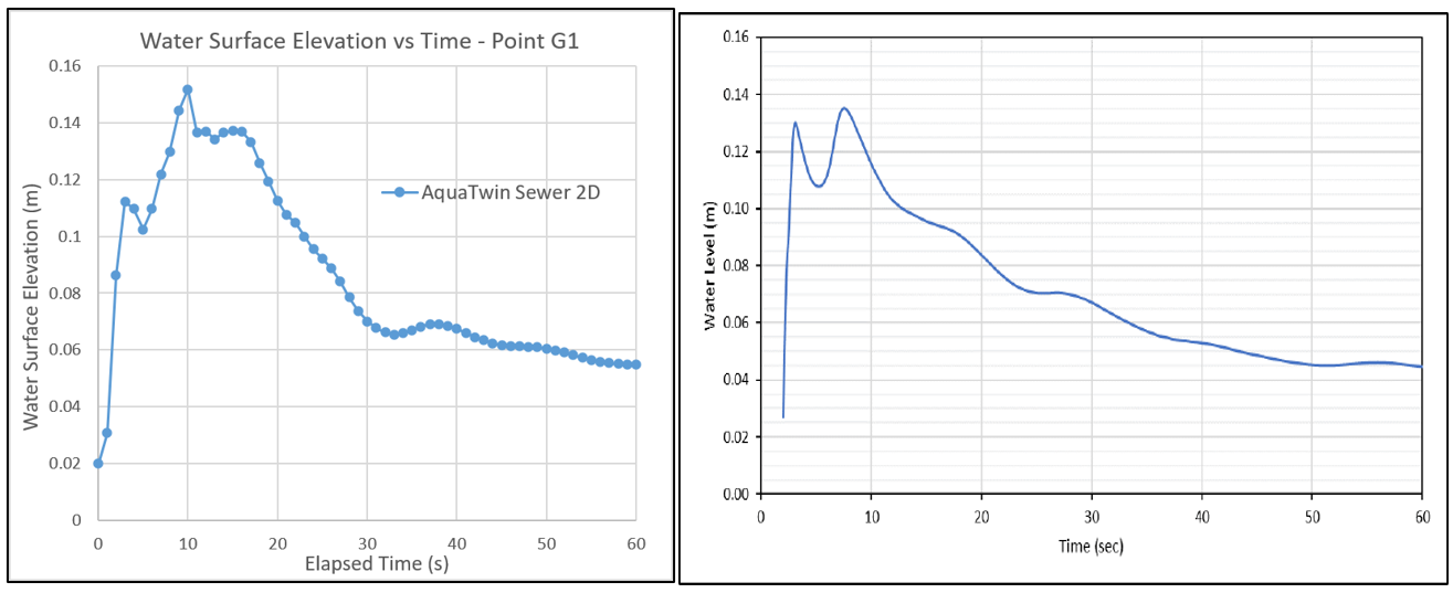
Figure A6.1) Point G1 WSE. Top Left: AquaTwin. Top right: SRH-2D, reproduced from Kramer (2021), p. 7-5.

Figure A6.2) Point G1 Velocity. Top Left: AquaTwin. Top right: SRH-2D, reproduced from Kramer (2021), p. 7-5.

Figure A6.3) Point G2 WSE. Top Left: AquaTwin. Top right: Ensemble, reproduced from Néelz and Pender (2013); as it appears in Kramer (2021), p. 7-6. Bottom Left: SRH-2D, reproduced from Kramer (2021), p. 7-6.

Figure A6.4) Point G2 Velocity. Top Left: AquaTwin. Top right: Ensemble, reproduced from Néelz and Pender (2013); as it appears in Kramer (2021), p. 7-7. Bottom Left: SRH-2D, reproduced from Kramer (2021), p. 7-7.
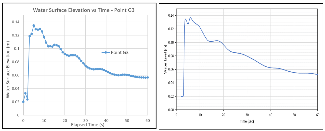
Figure A6.5) Point G3 WSE. Top Left: AquaTwin. Top right: SRH-2D, reproduced from Kramer (2021), p. 7-8.
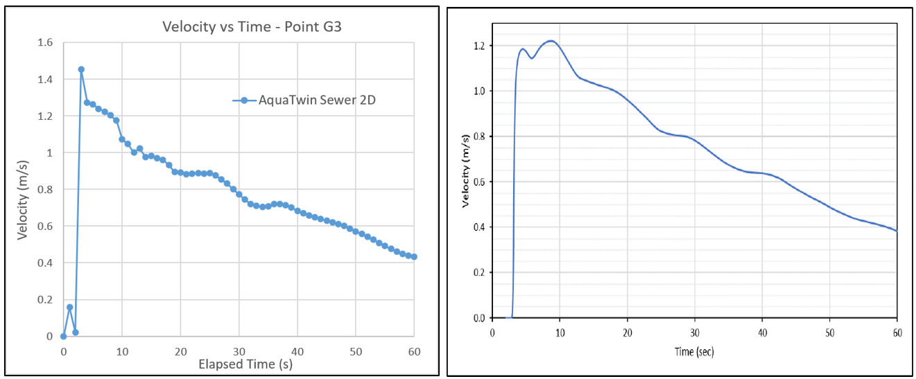
Figure A6.6) Point G3 Velocity. Top Left: AquaTwin. Top right: SRH-2D, reproduced from Kramer (2021), p. 7-8.

Figure A6.7) Point G4 WSE. Top Left: AquaTwin. Top right: Ensemble, reproduced from Néelz and Pender (2013); as it appears in Kramer (2021), p. 7-9. Bottom Left: SRH-2D, reproduced from Kramer (2021), p. 7-9.

Figure A6.8) Point G4 Velocity. Top Left: AquaTwin. Top right: Ensemble, reproduced from Néelz and Pender (2013); as it appears in Kramer (2021), p. 7-10. Bottom Left: SRH-2D, reproduced from Kramer (2021), p. 7-10.
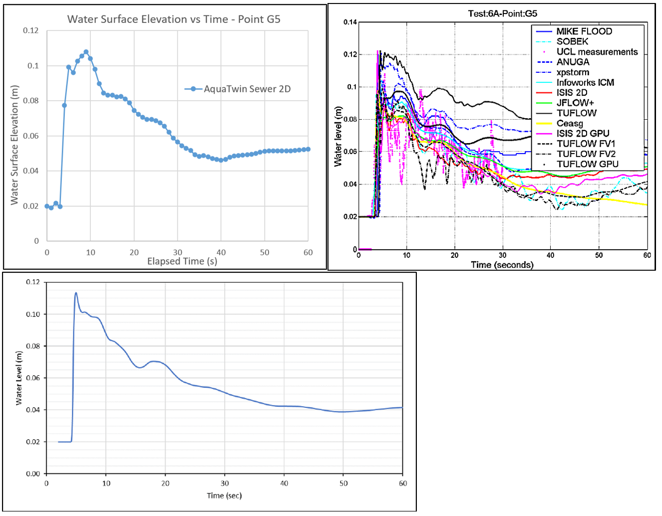
Figure A6.9) Point G5 WSE. Top Left: AquaTwin. Top right: Ensemble, reproduced from Néelz and Pender (2013); as it appears in Kramer (2021), p. 7-11. Bottom Left: SRH-2D, reproduced from Kramer (2021), p. 7-11.
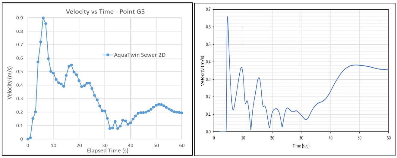
Figure A6.10) Point G5 Velocity. Top Left: AquaTwin. Top right: SRH-2D, reproduced from Kramer (2021), p. 7-12.
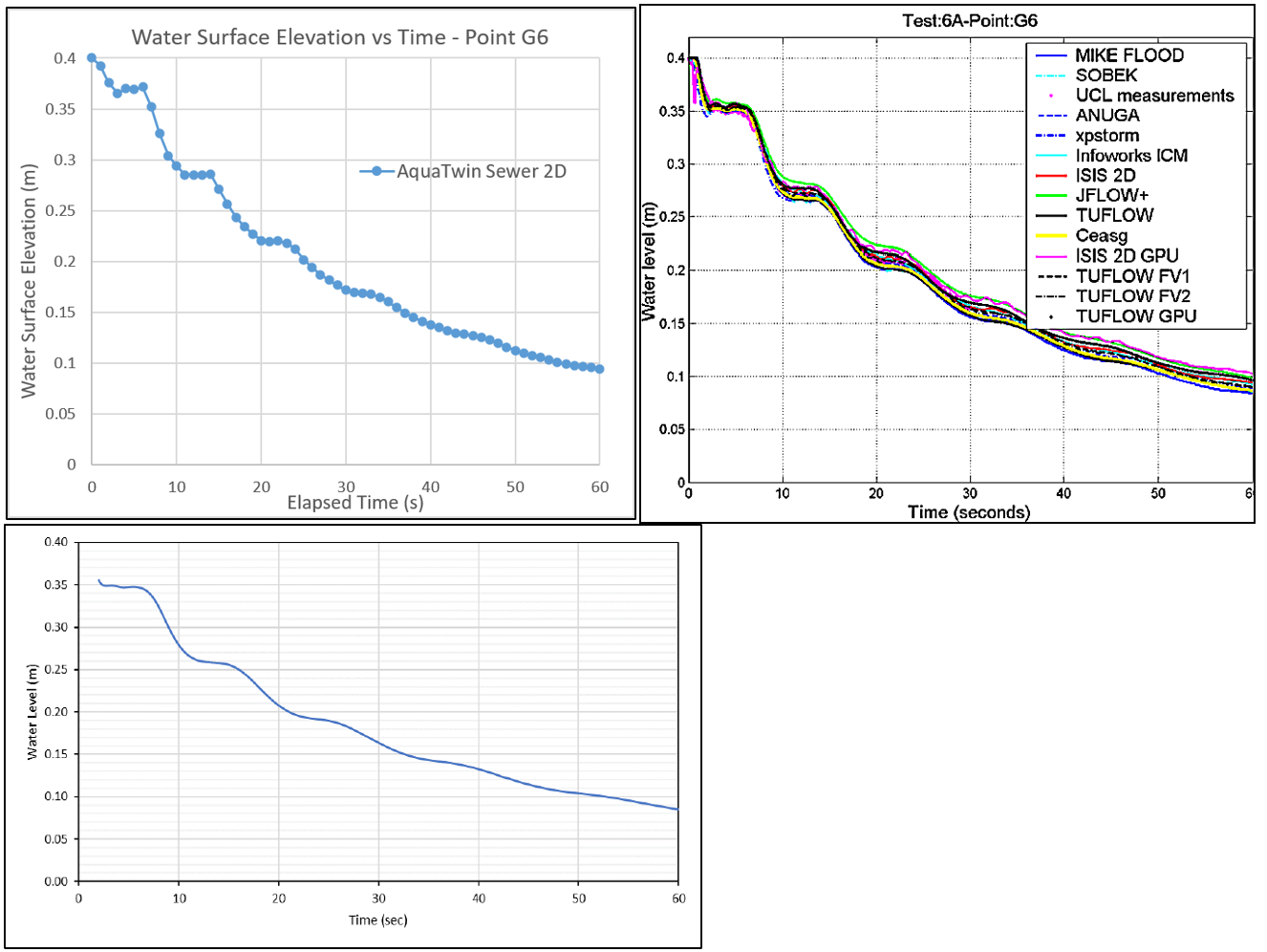
Figure A6.11) Point G6 WSE. Top Left: AquaTwin. Top right: Ensemble, reproduced from Néelz and Pender (2013); as it appears in Kramer (2021), p. 7-13. Bottom Left: SRH-2D, reproduced from Kramer (2021), p. 7-13.
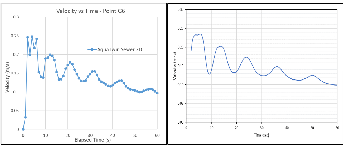
Figure A6.12) Point G6 Velocity. Left: AquaTwin. Right: SRH-2D, reproduced from Kramer (2021), p. 7-14.
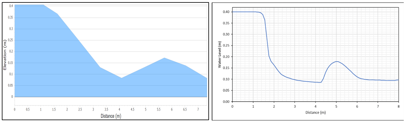
Figure A6.13) XS1 Maximum Water Level. Left: AquaTwin. Right: SRH-2D, reproduced from Kramer (2021), p. 7-16.
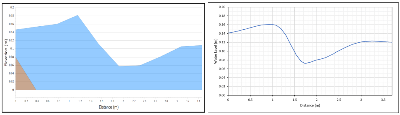
Figure A6.14) XS2 Maximum Water Level. Left: AquaTwin. Right: SRH-2D, reproduced from Kramer (2021), p. 7-17.
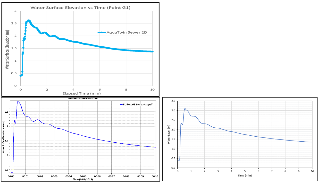
Figure A7.1) Point G1 WSE. Top Left: AquaTwin. Bottom Left: HEC-RAC FEQ, reproduced from Brunner (2018); as it appears in Kramer (2021), p. 7-21. Bottom Right: SRH-2D, reproduced from Kramer (2021), p. 7-21.

Figure A7.2) Point G1 Velocity. Top Left: AquaTwin. Bottom Left: HEC-RAC FEQ, reproduced from Brunner (2018); as it appears in Kramer (2021), p. 7-22. Bottom Right: SRH-2D, reproduced from Kramer (2021), p. 7-22.
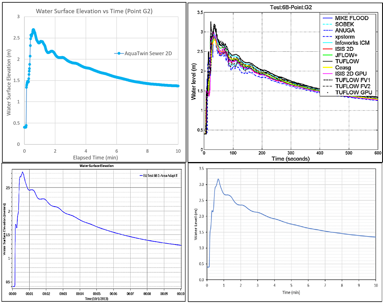
Figure A7.3) Point G2 WSE. Top Left: AquaTwin. Top Right: Ensemble, reproduced from Néelz and Pender (2013); as it appears in Kramer (2021), p. 7-23. Bottom Left: HEC-RAC FEQ, reproduced from Brunner (2018); as it appears in Kramer (2021), p. 7-23. Bottom Right: SRH-2D, reproduced from Kramer (2021), p. 7-23.

Figure A7.4) Point G2 Velocity. Top Left: AquaTwin. Top Right: Ensemble, reproduced from Néelz and Pender (2013); as it appears in Kramer (2021), p. 7-24. Bottom Left: HEC-RAC FEQ, reproduced from Brunner (2018); as it appears in Kramer (2021), p. 7-24. Bottom Right: SRH-2D, reproduced from Kramer (2021), p. 7-24.

Figure A7.5) Point G3 WSE. Top Left: AquaTwin. Bottom Left: HEC-RAC FEQ, reproduced from Brunner (2018); as it appears in Kramer (2021), p. 7-25. Bottom Right: SRH-2D, reproduced from Kramer (2021), p. 7-25.

Figure A7.6) Point G3 Velocity. Top Left: AquaTwin. Bottom Left: HEC-RAC FEQ, reproduced from Brunner (2018); as it appears in Kramer (2021), p. 7-26. Bottom Right: SRH-2D, reproduced from Kramer (2021), p. 7-26.

Figure A7.7) Point G4 WSE. Top Left: AquaTwin. Top Right: Ensemble, reproduced from Néelz and Pender (2013); as it appears in Kramer (2021), p. 7-27. Bottom Left: HEC-RAC FEQ, reproduced from Brunner (2018); as it appears in Kramer (2021), p. 7-27. Bottom Right: SRH-2D, reproduced from Kramer (2021), p. 7-27.

Figure A7.8) Point G4 Velocity. Top Left: AquaTwin. Top Right: Ensemble, reproduced from Néelz and Pender (2013); as it appears in Kramer (2021), p. 7-28. Bottom Left: HEC-RAC FEQ, reproduced from Brunner (2018); as it appears in Kramer (2021), p. 7-28. Bottom Right: SRH-2D, reproduced from Kramer (2021), p. 7-28.

Figure A7.9) Point G5 WSE. Top Left: AquaTwin. Top Right: Ensemble, reproduced from Néelz and Pender (2013); as it appears in Kramer (2021), p. 7-29. Bottom Left: HEC-RAC FEQ, reproduced from Brunner (2018); as it appears in Kramer (2021), p. 7-29. Bottom Right: SRH-2D, reproduced from Kramer (2021), p. 7-29.

Figure A7.10) Point G5 Velocity. Top Left: AquaTwin. Bottom Left: HEC-RAC FEQ, reproduced from Brunner (2018); as it appears in Kramer (2021), p. 7-30. Bottom Right: SRH-2D, reproduced from Kramer (2021), p. 7-30.
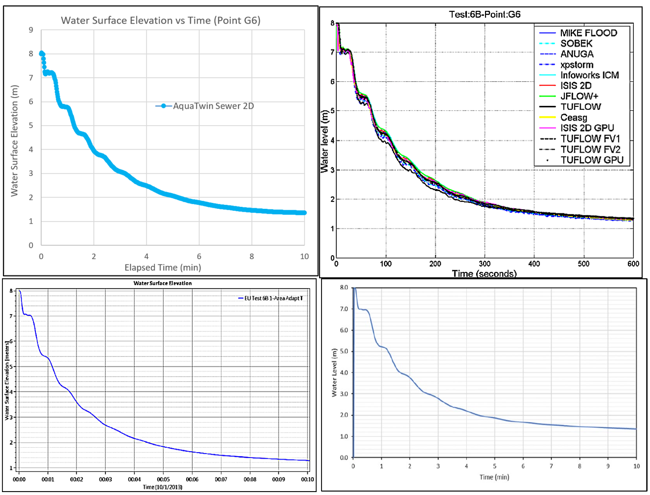
Figure A7.11) Point G6 WSE. Top Left: AquaTwin. Top Right: Ensemble, reproduced from Néelz and Pender (2013); as it appears in Kramer (2021), p. 7-31. Bottom Left: HEC-RAC FEQ, reproduced from Brunner (2018); as it appears in Kramer (2021), p. 7-31. Bottom Right: SRH-2D, reproduced from Kramer (2021), p. 7-31.
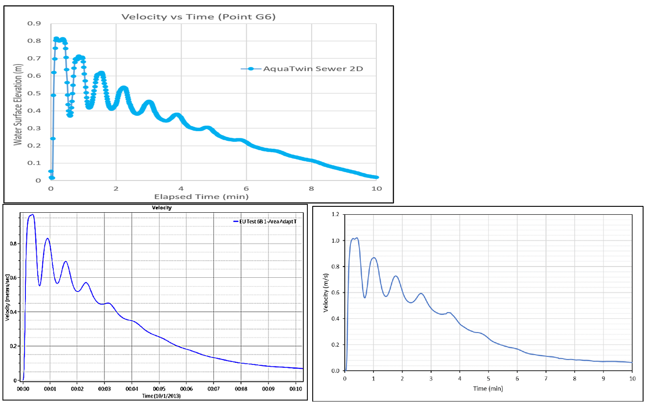
Figure A7.12) Point G6 Velocity. Top Left: AquaTwin. Bottom Left: HEC-RAC FEQ, reproduced from Brunner (2018); as it appears in Kramer (2021), p. 7-32. Bottom Right: SRH-2D, reproduced from Kramer (2021), p. 7-32.
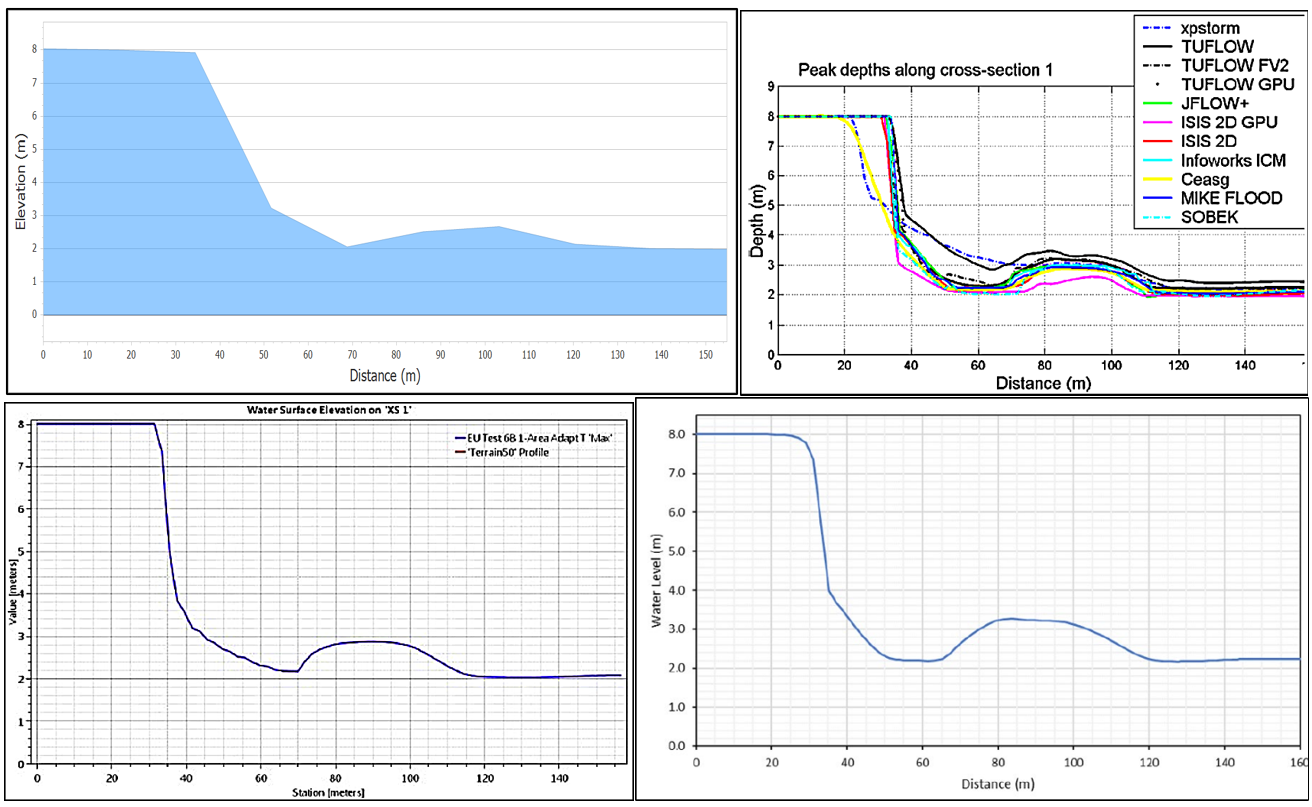
Figure A7.13) XS1 Maximum Water Level. Top Left: AquaTwin. Top Right: Ensemble, reproduced from Néelz and Pender (2013); as it appears in Kramer (2021), p. 7-34. Bottom Left: HEC-RAC FEQ, reproduced from Brunner (2018); as it appears in Kramer (2021), p. 7-34. Bottom Right: SRH-2D, reproduced from Kramer (2021), p. 7-34.
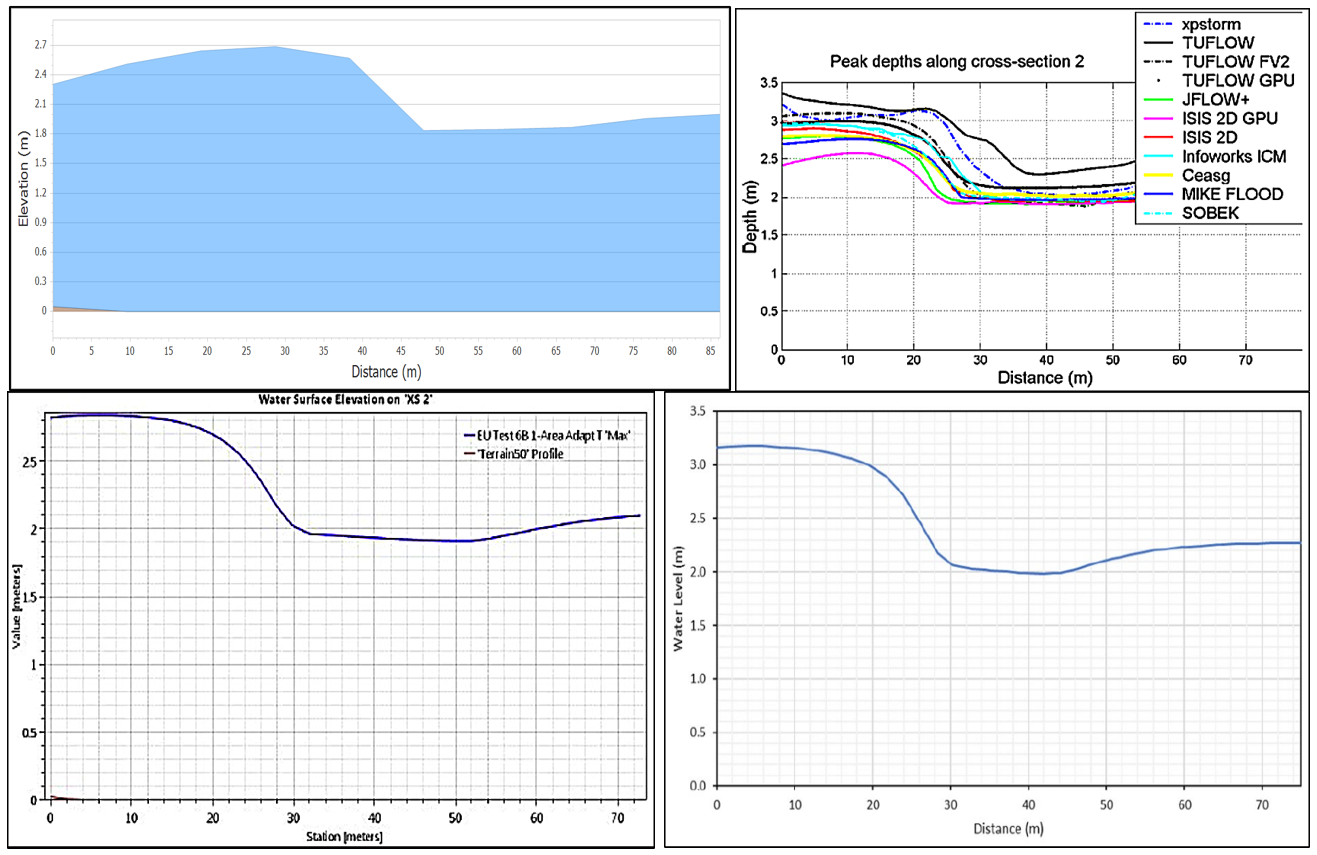
Figure A7.14) XS1 Maximum Water Level. Top Left: AquaTwin. Top Right: Ensemble, reproduced from Néelz and Pender (2013); as it appears in Kramer (2021), p. 7-36. Bottom Left: HEC-RAC FEQ, reproduced from Brunner (2018); as it appears in Kramer (2021), p. 7-36. Bottom Right: SRH-2D, reproduced from Kramer (2021), p. 7-36.
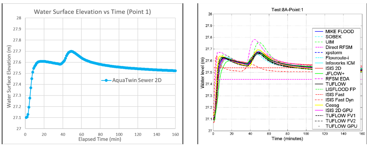
Figure A8.1) Point 1 WSE. Left: AquaTwin. Right: Ensemble, reproduced from Neelz & Pender, p.101.
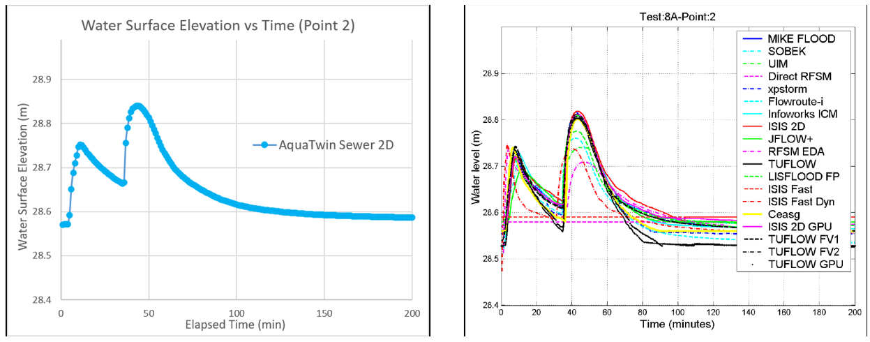
Figure A8.2) Point 2 WSE. Left: AquaTwin. Right: Ensemble, reproduced from Neelz & Pender, p.101.

Figure A8.3) Point 3 WSE. Left: AquaTwin. Right: Ensemble, reproduced from Neelz & Pender, p.102.

Figure A8.4) Point 6 WSE. Left: AquaTwin. Right: Ensemble, reproduced from Neelz & Pender, p.102.

Figure A8.5) Point 2 Velocity. Left: AquaTwin. Right: Ensemble, reproduced from Neelz & Pender, p.103.

Figure A8.6) Point 6 Velocity. Left: AquaTwin. Right: Ensemble, reproduced from Neelz & Pender, p.103.

Figure A8.7) Spatial extent of Max WSE > 0.2 m for a subset of the simulated domain (bounded by Point 1 on the right, Point 5 on the left). Top: Ensemble, reproduced from Néelz and Pender (2013), p. 104. Bottom: AquaTwin.

Figure A9.1) Manhole Flooding. Left: AquaTwin. Right: Ensemble, reproduced from Neelz & Pender, p.110.

Figure A9.2) Point 1 WSE. Left: AquaTwin. Right: Ensemble, reproduced from Neelz & Pender, p.111.

Figure A9.3) Point 2 WSE. Left: AquaTwin. Right: Ensemble, reproduced from Neelz & Pender, p.111.

Figure A9.4) Point 3 WSE. Left: AquaTwin. Right: Ensemble, reproduced from Neelz & Pender, p.112.

Figure A9.5) Point 3 Velocity. Left: AquaTwin. Right: Ensemble, reproduced from Neelz & Pender, p.112.